Welcome
Dear Students,
Welcome to the programming course in theoretical chemistry. This class builds on the bachelor lecture "Programming Course for Chemists" and assumes that you are already familiar with the basic principles of Python and the numerical algorithms explained there.
According to current planning, the lecture will take place on
- every Monday from 10:15 to 11:45
and
- every Thursday from 12:15 to 13:45.
Syllabus
A preliminary syllabus is shown below. This can and will be continuously updated throughout the semester according to the progress of the lecture.
| Week | Weekday | Date | Type | Topic |
|---|---|---|---|---|
| 1 | Mon. | April 17 | Lecture | Fundamentals I |
| 1 | Thur. | April 20 | Lecture | Fundamentals II |
| 2 | Mon. | April 24 | Lecture | SymPy: Basics |
| 2 | Thur. | April 27 | Lecture | SymPy: Applications |
| 4 | Mon. | May 8 | Lecture | Overlap Integral I |
| 4 | Thur. | May 11 | Exercise | Exercise 0 |
| 5 | Mon. | May 15 | Lecture | Overlap Integral II |
| 6 | Mon. | May 22 | Lecture | Molecule Class I |
| 6 | Thur. | May 25 | Lecture | Molecule Class II |
| 7 | Thur. | June 1 | Exercise | Exercise 1 |
| 8 | Mon. | June 5 | Lecture | Nuclear Attraction Integral I |
| 9 | Mon. | June 12 | Lecture | Optimization |
| 9 | Thur. | June 15 | Lecture | Nuclear Attraction Integral II |
| 10 | Mon. | June 19 | Lecture | Electron Repulsion Integral I |
| 10 | Thur. | June 22 | Exercise | Exercise 2 |
| 11 | Mon. | June 26 | Lecture | Electron Repulsion Integral II |
| 11 | Thur. | June 29 | Lecture ] Hartree-Fock I | |
| 12 | Mon. | July 3 | Lecture | Hartree-Fock II |
| 12 | Thur. | July 6 | Lecture | Configuration Interaction Singles |
| 13 | Mon. | July 10 | Exercise | Exercise 3 |
| 13 | Thur. | July 13 | Lecture | Second Quantization |
| 14 | Mon. | July 17 | Lecture | Full Configurational Interaction I |
| 14 | Thur. | July 20 | Lecture | Full Configurational Interaction II |
Technical notes
Python Distribution
We highly recommend to use the Anaconda or the Mamba Python distribution. Between these two options, Mamba is the top choice since it is much faster than Anaconda. Follow one of the following instructions to install Anaconda or Mamba. Do NOT install both distributions! Your Python version for this class should be 3.5 or higher.
Anaconda
Follow the installation guide for your operating system here.
Mamba
- Download Mambaforge installer acoording to your operating system here.
- Execute the installer:
-
Unix-like platforms (Mac OS & Linux):
Open the terminal and call
bash [Mambaforge-installer].shwhere
[Mambaforge-installer]should be replaced by your installer, e.g.Mambaforge-Linux-x86_64orMambaforge-MacOSX-x86_64. -
Windows:
Double click the installer on the file browser.
Integrated Development Environment (IDE) or Editor recommendations
Although it is possible to write Python code using a conventional text editor, an integrated development environment can boost your programming experience greatly. Therefore, we shall show you some recommendations of IDEs and specialised editors here.
-
- will be automatically available after you have installed Anaconda/Miniconda.
- if you are not yet familiar with Jupyter notebooks, you can find many tutorials in the web, e.g. Tutorial.
-
- is a full Python IDE with the focus on scientific development.
- will be automatically installed if you install the full Anaconda package.
-
- is a more lightweight text editor for coding purposes and one of the most used ones.
- Although it is officially not a real IDE, it has almost all features of an IDE.
-
- commercial (free for students) IDE with a lot of functionalities.
- is usually more suitable for very large and complex Python projects and can be too cumbersome for small projects like the ones used here in the lecture.
-
Vim/NeoVim
- command-line text editor which is usually pre installed on all unix-like computers.
- can be very unwieldy at the beginning, since Vim has a very large number of keyboard shortcuts and is not as beginner friendly as a typical IDE or Jupyter notebooks.
- is extremely configurable and can be adapted with a little effort to a very extensive and comfortable editor.
- still one of the most used editors.
Dependencies
During the lecture we will use different Python libraries, which can be conveniently installed via a package manager. The Anaconda distribution comes with the package manager conda while the Mamba distribution has mamba. Please install these packages by executing the following commands in your terminal.
Note: If you are using Windows, execute the commands in Anaconda Prompt or Miniforge Prompt that comes with your Anaconda or Mambaforge installation.
| Library | conda | mamba |
|---|---|---|
| NumPy | conda install numpy | mamba install numpy |
| Matplotlib | conda install -c conda-forge matplotlib | mamba install matplotlib |
| SciPy | conda install scipy | mamba install scipy |
| SymPy | conda install sympy | mamba install sympy |
| Jupyter | Preinstalled with Anaconda | mamba install notebook |
| pytest | conda install pytest | mamba install pytest |
| ipytest | conda install -c conda-forge ipytest | mamba install ipytest |
| Hypothesis | conda install -c conda-forge hypothesis | mamba install hypothesis |
Why Python?
Popularity
Python is one of the most widely used programming languages and is particularly beginner-friendly.
The following figure shows the popularity of some programming languages.
 Popularity of common programming languages. The popularities are taken
from the PYPL index
Popularity of common programming languages. The popularities are taken
from the PYPL index
Requires often fewer lines of code and less work
Python often requires significantly fewer lines of code to implement
the same algorithms than compiled languages such as Java or C/C++.
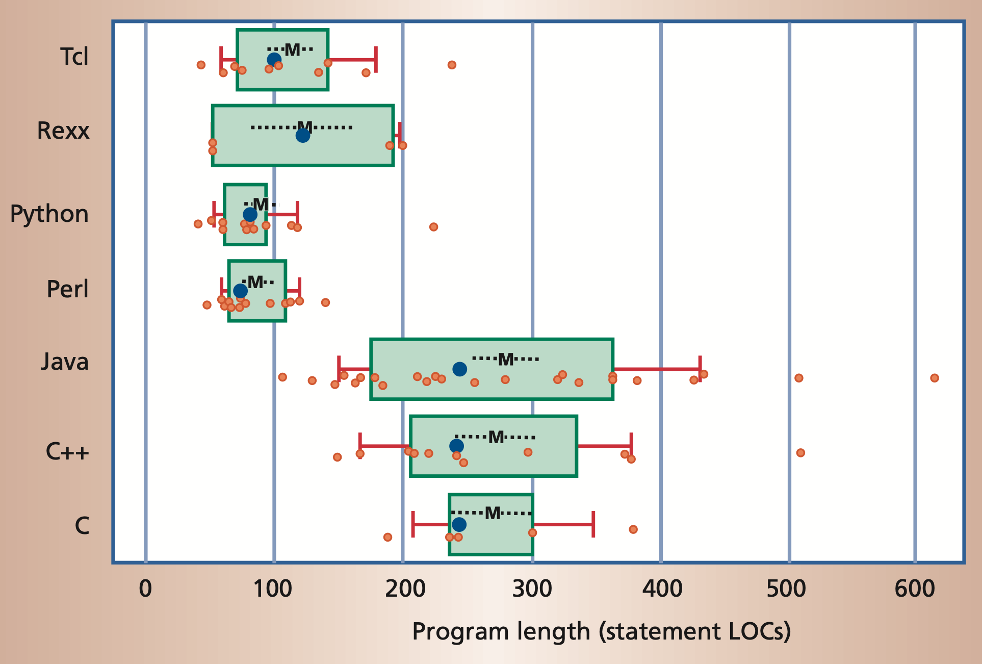 Program length, measured in number of noncomment source lines of code
(LOC).
Program length, measured in number of noncomment source lines of code
(LOC).
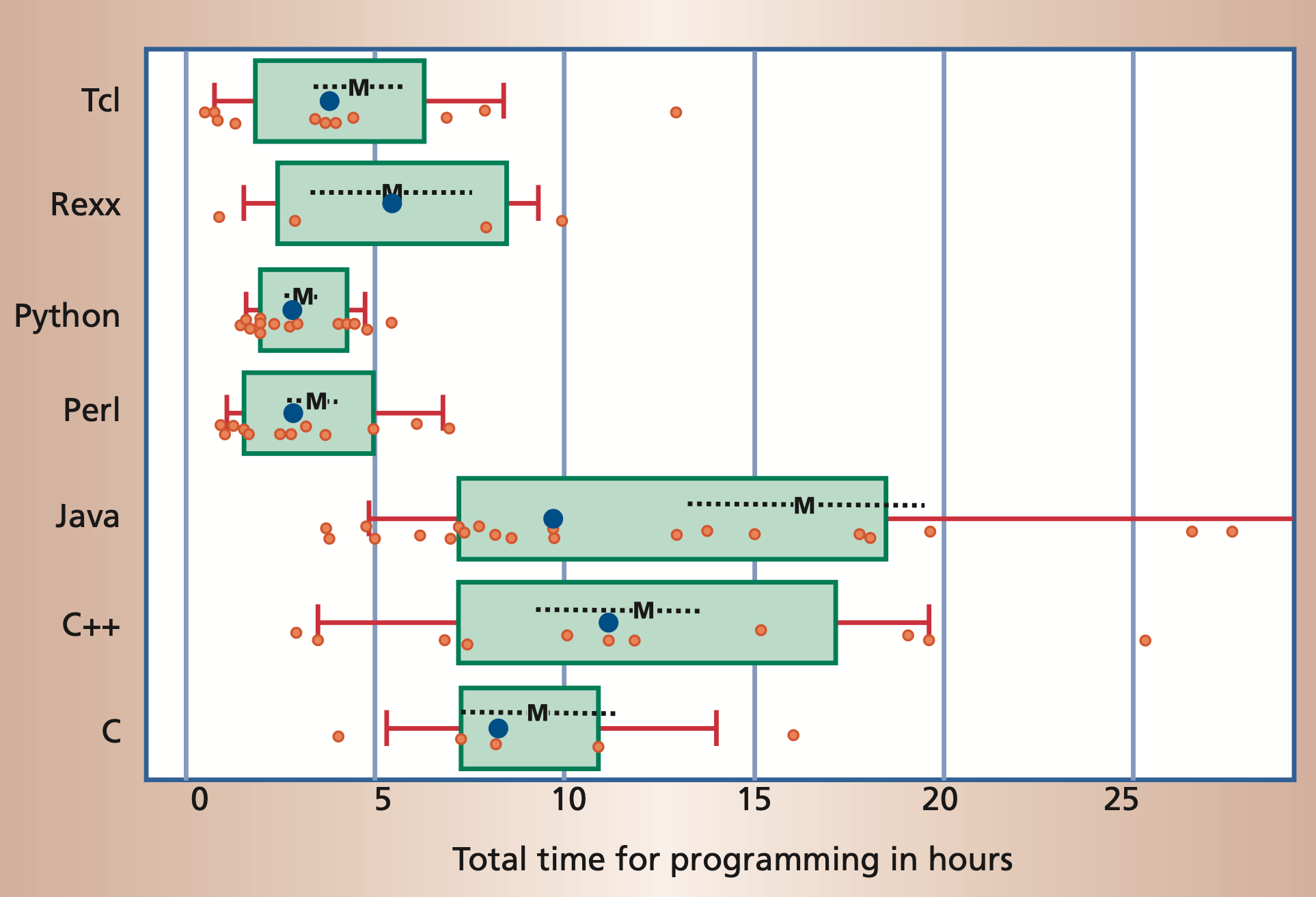
Moreover, it is often possible to accomplish the same task in significantly
less time in a scripting language than it takes using a compiled language.
But Python is slow!?
A common argument that is raised against using Python is that it is a comparatively slow language. There is some truth to this statement. Therefore, we want to understand one of the reasons why this is so and then explain why (in most cases) this is not a problem for us.
Python is an interpreted language.
Python itself is a C program that reads the source code of a text file, interprets it and executes it. This is in contrast to a compiled language like C, C++, Rust, etc. where the source code is compiled to machine code. The compiler has the ability to do lots of optimizations to the code which leads to a shorter runtime. This behavior can be shown by a simple example. Let's assume we have a naïve implementation to sum up all odd numbers up to 100 million:
s = 0
for i in range(100_000_000):
    if i % 2 == 1:
        s += i
This code takes about 8 seconds on my computer (M1 mac) to execute. Now we can implement the same algorithm in a compiled language to see the impact of the compiler. The following listing is written in a compiled language (Rust), but the details of this code and the programming language do not matter at this point:
#![allow(unused)]
fn main() {
let mut s: usize = 0;
for i in 0..100_000_000 {
    if i % 2 == 1 {
        s += i;
    }
}
}
This code has actually no runtime at all and evaluates instantaneously.
The compiler is smart enough to understand that everything can be
computed at compile time and just inserts the value for the variable
s. This now makes it clear that compiled languages can make use of
methods that interpreted languages lack simply by virtue of their
approach. However, we have seen before that compiled languages usually
require more lines of code and more work. In addition, there are usually
much more concepts to learn.
Python can be very performant
During this lecture we will often use Python libraries like NumPy or Scipy for mathematical algorithms and linear algebra in particular. These packages bring two big advantages. On the one hand they allow the use of complicated algorithms very easily and on the other hand these packages are written in compiled languages like C or Fortran. This way we can benefit from the performance advantages without having to learn another possibly more complicated language.
How to interact with this website
This section gives an introduction on how to interact with the lecture notes. These are organized into chapters. Each chapter is a separate page. Chapters are nested into a hierarchy of sub-chapters. Typically, each chapter will be organized into a series of headings to subdivide a chapter.
Navigation
There are several methods for navigating through the chapters of a book.
The sidebar on the left provides a list of all chapters. Clicking on any of the chapter titles will load that page.
The sidebar may not automatically appear if the window is too narrow, particularly on mobile displays. In that situation, the menu icon (three horizontal bars) at the top-left of the page can be pressed to open and close the sidebar.
The arrow buttons at the bottom of the page can be used to navigate to the previous or the next chapter.
The left and right arrow keys on the keyboard can be used to navigate to the previous or the next chapter.
Top menu bar
The menu bar at the top of the page provides some icons for interacting with the notes.
| Icon | Description |
|---|---|
| Opens and closes the chapter listing sidebar. | |
| Opens a picker to choose a different color theme. | |
| Opens a search bar for searching within the book. | |
| Instructs the web browser to print the set of notes. |
Tapping the menu bar will scroll the page to the top.
Search
The lecture notes have a built-in search system.
Pressing the search icon () in the menu bar or pressing the S key on the keyboard will open an input box for entering search terms.
Typing any terms will show matching chapters and sections in real time.
Clicking any of the results will jump to that section. The up and down arrow keys can be used to navigate the results, and enter will open the highlighted section.
After loading a search result, the matching search terms will be highlighted in the text.
Clicking a highlighted word or pressing the Esc key will remove the highlighting.
Code blocks
Code blocks contain a copy icon , that copies the code block into your local clipboard.
Here's an example:
print("Hello, World!")
We will often use the assert statement in code listings to show you
the value of a variable. Since the code blocks in this document are not
interactive (you can not simply execute them in your browser), it is
not possible to print the value of the variable to the screen.
Therefore, we ensure for you that all code blocks in these lecture notes
run without errors and in this way we can represent the value of a
variable through the use of assert.
The following code block for example shows that the variable a has
the value 2:
a = 2
assert a == 2
If the condition would evaluate to False, the assert statement would
raise an AssertionError.
Fundamentals
In the following sections, we will explain the concept of bitwise operators after laying the necessary foundations. Our goal is to show what bitwise operators do and what they can be used for. Afterwards, we also want to show the possibility and importance of unit tests. At the end of this chapter you should be able to answer the following questions:
- How are numbers represented in the computer?
- What is the difference in the representation between signed and unsigned integers?
- What are bitwise operators? Can you name and explain a few examples?
- What are unit tests? Why are they important?
Binary Numbers
When working with any kind of digital electronics, it is important to understand that numbers are represented by two levels in these devices, which stand for one or zero. The number system based on ones and zeroes is called the binary system (because there are only two possible digits). Before discussing the binary system, a review of the decimal system (ten possible digits) is helpful, because many of the concepts of the binary system will be easier to understand when introduced alongside their decimal counterparts.
Decimal System
As a human on earth, you should have some familiarity with the decimal system. For instance, to represent the positive integer one hundred and twenty-five as a decimal number, we can write (with the postive sign implied):
$$ 125_{10} = 1 \cdot 100 + 2 \cdot 10 + 5 \cdot 1 = 1 \cdot 10^2 + 2 \cdot 10^1 + 5 \cdot 10^0 $$
The subscript 10 denotes the number as a base 10 (decimal) number.
There are some important observations:
- To multiply a number by 10, you can simply shift it to the left by one digit, and fill in the rightmost digit with a 0 (moving the decimal place by one to the right).
- To divide a number by 10, you can simply shift it to the right by one digit (moving the decimal place by one to the left).
- To see how many digits a number has, you can simply take the logarithm (base 10) of the absolute value of the number, and add 1 to it. The integral part of the result will be the number of digits. For instance, \(\log_{10}(33) + 1 = 2.5.\)
Binary System (of positive integers)
Binary representations of positive integers can be understood in the same way as their decimal counterparts. For example
$$ 86_{10}=1 \cdot 64+0 \cdot 32+1 \cdot 16+0 \cdot 8+1 \cdot 4+1 \cdot 2+0 \cdot 1 $$
This can also be written as:
$$ 86_{10}=1 \cdot 2^{6} +0 \cdot 2^{5}+1 \cdot 2^{4}+0 \cdot 2^{3}+1 \cdot 2^{2}+1 \cdot 2^{1}+0 \cdot 2^{0} $$ or
$$ 86_{10}=1010110_{2} $$
The subscript 2 denotes a binary number. Each digit in a binary number is called a bit. The number 1010110 is represented by 7 bits. Any number can be broken down this way by finding all of the powers of 2 that add up to the number in question (in this case \(2^6\), 2\(^4\), 2\(^2\) and 2\(^1\)). You can see this is exactly analogous to the decimal deconstruction of the number 125 that we have done earlier. Likewise we can make a similar set of observations:
- To multiply a number by 2, you can simply shift it to the left by one digit, and fill in the rightmost digit with a 0.
- To divide a number by 2, you can simply shift it to the right by one digit.
- To see how many digits a number has, you can simply take the logarithm (base 2) of the number, and add 1 to it. The integral part of the result is the number of digits. For instance, \(\log_{2}(86) + 1 = 7.426.\) The integral part of that is 7, so 7 digits are needed. With \(n\) digits, \(2^n\) unique numbers (from 0 to \(2^n - 1\)) can be represented. If \(n=8\), 256 (\(=2^8\)) numbers can be represented (0-255).
This counter shows how to count in binary from zero through thirty-one.
Binary System of Signed Integers
Since digital electronics only have access to two levels standing for 0 and 1, we will not be able to use a minus sign (\(-\)) for representing negative numbers. There are a few common ways to represent negative binary numbers by only using ones and zeros, which we will discuss in the following subsections.
Note: Unlike other programming languages, where different types of integers exist (signed, unsigned, different number of bits), Python only has one integer type (
int). This is a signed integer type with arbitrary precision. This means, the integer does not have a fixed number of bits to represent the number, but will dynamically use as many bits as needed to represent the number. Therefore, integer overflows cannot occur in Python. This doesn't hold forfloats, which have fixed size of 64 bit and can overflow.
Sign and Magnitude
The most significant bit (MSB) determines if the number is positive (MSB is 0) or negative (MSB is 1). All the other bits are the so called magnitude bits. This means that a 8 bit signed integer can represent all numbers from -127 to 127 (\(-2^6\) to \(2^6\)). Except for the MSB, all positive and negative numbers share the same representation.

Visualization of the Sign and Magnitude representation of the decimal number +13.
In the case of a negative number, the only difference is that the first bit (the MSB) is inverted, as shown in the following Scheme.

Visualization of the Sign and Magnitude representation of the decimal number -31
Although this representation seems very intimate and simple, several problems asscociated to the sign bit arise:
- There are two ways to represent zero,
0000 0000and1000 0000. - Addition and subtraction require different behaviors depending on the sign bit.
- Comparisons (e.g. greater, less, ...) also require inspection of the sign bit.
This approach is directly comparable to the common way of showing a sign (placing a "+" or "−" next to the number's magnitude). This kind of representation was only used in early binary computers and was replaced by representations that we will discuss in the following.
Ones' Complement
To overcome the limitations of the Sign and Magnitude representation, another representation was developed with the following idea in mind: One wants to flip the sign of an integer by inverting all its bits.
This inversion is also known as taking the complement of the bits. The implication of this idea is, that the first bit, the MSB, also represents just the sign as in the Sign and Magnitude case. However, the decimal value of all other bits are now dependent of the MSB bit state. It might be easier to understand this behavior by a simple example that outlines the motivation again.
We want that our binary representation behaves like:

The advantage of this representation is that for adding two numbers, one can do a conventional binary addition, but it is then necessary to do an end-around carry: that is, add any resulting carry back into the resulting sum. To see why this is necessary, consider the following example showing the case of the following addition $$ −1_{10} + 2_{10} $$
or
$$ 1111 1110_2 + 0000 0010_2 $$

In the previous example, the first binary addition gives 00000000, which
is incorrect. The correct result (00000001) only appears when the carry
is added back in.
A remark on terminology: The system is referred to as ones' complement because the negation of a positive value x (represented as the bitwise NOT of x, we will discuss the bitwise NOT in the following sections) can also be formed by subtracting x from the ones' complement representation of zero that is a long sequence of ones (−0).
Two's Complement
In the two's complement representation, a negative number is represented by the bit pattern corresponding to the bitwise NOT (i.e. the "complement") of the positive number plus one, i.e. to the ones' complement plus one. It circumvents the problems of multiple representations of 0 and the need for the end-around carry of the ones' complement representation.
This can also be thought of as the most significant bit representing the inverse of its value in an unsigned integer; in an 8-bit unsigned byte, the most significant bit represents the number 128, where in two's complement that bit would represent −128.

In two's-complement, there is only one zero, represented as 00000000. Negating a number (whether negative or positive) is done by inverting all the bits and then adding one to that result.
Addition of a pair of two's-complement integers is the same as addition of a pair of unsigned numbers. The same is true for subtraction and even for the (N) lowest significant bits of a product (value of multiplication). For instance, a two's-complement addition of 127 and −128 gives the same binary bit pattern as an unsigned addition of 127 and 128, as can be seen from the 8-bit two's complement table.

Two's complement is the representation that Python uses for it's type
int.
Logic Gates
Truth tables show the result of combining inputs using a given operator.
NOT Gate
The NOT gate, a logical inverter, has only one input. It reverses the logic state. If the input is 0, then the output is 1. If the input is 1, then the output is 0.
| INPUT | OUTPUT |
|---|---|
| 0 | 1 |
| 1 | 0 |
AND Gate
The AND gate acts in the same way as the logical "and" operator. The following truth table shows logic combinations for an AND gate. The output is 1 only when both inputs are 1, otherwise, the output is 0.
| A | B | Output |
|---|---|---|
| 0 | 0 | 0 |
| 0 | 1 | 0 |
| 1 | 0 | 0 |
| 1 | 1 | 1 |
OR Gate
The OR gate behaves after the fashion of the logical inclusive "or". The output is 1 if either or both of the inputs are 1. Only if both inputs are 0, then the output is 0.
| A | B | Output |
|---|---|---|
| 0 | 0 | 0 |
| 0 | 1 | 1 |
| 1 | 0 | 1 |
| 1 | 1 | 1 |
NAND Gate
The NAND gate operates as an AND gate followed by a NOT gate. It acts in the manner of the logical operation "and" followed by negation. The output is 0 if both inputs are 1. Otherwise, the output is 1.
| A | B | Output |
|---|---|---|
| 0 | 0 | 1 |
| 0 | 1 | 1 |
| 1 | 0 | 1 |
| 1 | 1 | 0 |
NOR Gate
The NOR gate is a combination of OR gate followed by a NOT gate. Its output is 1 if both inputs are 0. Otherwise, the output is 0.
| A | B | Output |
|---|---|---|
| 0 | 0 | 1 |
| 0 | 1 | 0 |
| 1 | 0 | 0 |
| 1 | 1 | 0 |
XOR Gate
The XOR (exclusive-OR) gate acts in the same way as the logical "either/or." The output is 1 if either, but not both, of the inputs are 1. The output is 0 if both inputs are 0 or if both inputs are 1. Another way of looking at this circuit is to observe that the output is 1 if the inputs are different, but 0 if the inputs are the same.
| A | B | Output |
|---|---|---|
| 0 | 0 | 0 |
| 0 | 1 | 1 |
| 1 | 0 | 1 |
| 1 | 1 | 0 |
XNOR Gate
The XNOR (exclusive-NOR) gate is a combination of XOR gate followed by a NOT gate. Its output is 1 if the inputs are the same, and 0 if the inputs are different.
| A | B | Output |
|---|---|---|
| 0 | 0 | 1 |
| 0 | 1 | 0 |
| 1 | 0 | 0 |
| 1 | 1 | 1 |
To see these gates in action, you can try the game Digital Logic Sim, which is explained in https://youtu.be/QZwneRb-zqA.
Bitwise Operators
Bitwise operators are used to manipulate the states of bits directly. In Python (>3.5), 6 bitwise operators are defined:
| Operator | Name | Example | Output (x=7, y=2) |
|---|---|---|---|
<< | left bitshift | x << y | 28 |
>> | right bitshift | x >> y | 1 |
& | bitwise and | x & y | 2 |
| | bitwise or | x | y | 7 |
~ | bitwise not | ~x | -8 |
^ | bitwise xor | x ^ y | 5 |
Left Bitshift
Returns x with the bits shifted to the left by y places (and new bits on the right-hand-side are zeros). This is the same as multiplying \(x\) by \(2^y\).
The easiest way to visualize this operation is to consider a number that consists of only a single 1 in binary representation. If we now simply shift a 1 to the left three times in succession, we get the following:
assert (1 << 1) == 2  # ..0001 => ..0010
assert (2 << 1) == 4  # ..0010 => ..0100
assert (4 << 1) == 8  # ..0100 => ..1000
But we can also do this operation with just one call:
assert (1 << 3) == 8 # ..0001 => ..1000
Of course, we can also apply this operation to any other number:
assert (3 << 2) == 12 # ..0011 => ..1100
Right Bitshift
Returns x with the bits shifted to the right by y places. This is the same as dividing \(x\) by \(2^y\).
assert (8 >> 1) == 4 # ..1000 => ..0100
assert (4 >> 1) == 2 # ..0100 => ..0010
assert (2 >> 1) == 1 # ..0010 => ..0001
As we did with the bit shift to the left side, we can also shift a bit multiple times to the right:
assert (8 >> 3) == 1 # ..1000 => ..0001
Or apply the operator to any other number that is not a multiple of 2.
assert (11 >> 2) == 2 # ..1011 => ..0010
Bitwise AND
Does a "bitwise and". Each bit of the output is 1 if the corresponding bit of \(x\) AND \(y\) is 1, otherwise it is 0.
assert (1 & 2) == 0  # ..0001 & ..0010 => ..0000
assert (7 & 5) == 5  # ..0111 & ..0101 => ..0101
assert (12 & 3) == 0 # ..1100 & ..0011 => ..0000
Bitwise OR
Does a "bitwise or". Each bit of the output is 0 if the corresponding bit of \(x\) OR \(y\) is 0, otherwise it's 1.
assert (1 | 2) == 3   # ..0001 & ..0010 => ..0011
assert (7 | 5) == 7   # ..0111 & ..0101 => ..0111
assert (12 | 3) == 15 # ..1100 & ..0011 => ..1111
Bitwise NOT
Returns the complement of \(x\) - the number you get by switching each 1 for a 0 and each 0 for a 1. This is the same as \(-x - 1\).
assert ~0 == -1
assert ~1 == -2
assert ~2 == -3
assert ~3 == -4
Bitwise XOR
Does a "bitwise exclusive or". Each bit of the output is the same as the corresponding bit in \(x\) if that bit in \(y\) is 0, and it is the complement of the bit in x if that bit in y is 1.
assert (1 ^ 2) == 3   # ..0001 & ..0010 => ..0011
assert (7 ^ 5) == 2   # ..0111 & ..0101 => ..0010
assert (12 ^ 3) == 15 # ..1100 & ..0011 => ..1111
Arithmetic Operators
Arithmetic operators are used to perform mathematical operations like addition, subtraction, multiplication and division. In Python (>3.5), 7 arithmetic operators are defined:
| Operator | Name | Example | Output (x=7, y=2) |
|---|---|---|---|
+ | Addition | x + y | 9 |
- | Subtraction | x - y | 5 |
* | Multiplication | x * y | 14 |
/ | Division | x / y | 3.5 |
// | Floor division | x // y | 3 |
% | Modulus | x % y | 1 |
** | Exponentiation | x ** y | 49 |
Addition
The + (addition) operator yields the sum of its arguments.
The arguments must either both be numbers or both be sequences of the same type. Only in the former case, the numbers are converted to a common type and a arithmetic addition is performed. In the latter case, the sequences are concatenated, e.g.
a = [1, 2, 3]
b = [4, 5, 6]
assert (a + b) == [1, 2, 3, 4, 5, 6]
Subtraction
The - (subtraction) operator yields the difference of its arguments.
The numeric arguments are first converted to a common type.
Note: In contrast to the addition, the subtraction operator cannot be applied to sequences.
Multiplication
The * (multiplication) operator yields the product of its arguments.
The arguments must both be numbers, or alternatively, one argument must be an integer while the other must be a sequence.
In the former case, the numbers are converted to a common type and then multiplied together.
In the latter case, sequence repetition is performed; e.g.
a = [1, 2]
assert (3 * a) == [1, 2, 1, 2, 1, 2]
Note: a negative repetition factor yields an empty sequence; e.g.
a = 3 * [1, 2]
assert (-2 * a) == []
Division & Floor division
The / (division) and // (floor division) operators yield the
quotient of their arguments.
The numeric arguments are first converted to a common type.
Beaware that division of integers yields a float,
while floor division of integers results in an integer.
The result of the floor division operator is that of mathematical division
with the floor function applied to the result.
Division by zero raises a ZeroDivisionError exception.
Modulus
The % (modulo) operator yields the remainder from the division of the first argument by the second.
The numeric arguments are first converted to a common type.
A zero right argument raises the ZeroDivisionError exception.
The arguments may even be floating point numbers, e.g.,
import math
assert math.isclose(3.14 % 0.7, 0.34)
assert math.isclose(3.14, 4*0.7 + 0.34)
The modulo operator always yields a result with the same sign as its second operand (or zero); the absolute value of the result is strictly smaller than the absolute value of the second operand.
Note: As you may have noticed in the listing above, we did not use the comparison operator
==to test the equality of two floats. Instead we imported themathpackage and used the built-in isclose function. If you want to learn more about float representation errors, you may find some useful information in this blog post.
Note: If you need both the quotient and the remainder, instead of performing a floor division followed by a modulus evaluation, you should use the built-in
divmodfunction.
Exponentiation
The ** (power) operator has the same semantics as the
built-in pow() function, when called with two arguments,
it yields the left argument raised to the power of the right argument.
Numeric arguments are first converted to a common type, the result
type is that of the arguments after coercion.
If the result is not expressible in that type,
(as in raising an integer to a negative power)
the result is expressed as a float (or complex).
In an unparenthesized sequence of power and unary operators, the operators are evaluated from right to left
(this does not constrain the evaluation order for the operands), e.g.
assert 2**2**3 == 2**(2**3) == 2**8 == 256
Implementation: Arithmetic Operators
All arithmetic operators can be implemented using bitwise operators. While addition and subtraction are implemented through hardware, the other operators are often realized via software. In this section, we shall implement multiplication and division for positive integers using addition, subtraction and bitwise operators.
Implementation: Multiplication
The multiplication of integers may be thought as repeated addition; that is, the multiplication of two numbers is equivalent to the following sum: $$ A \cdot B = \sum_{i=1}^{A} B $$ Following this idea, we can implement a naïve multiplication:
def naive_mul(a, b):
    r = 0
    for i in range(0, a):
        r += b
    return r
Although we could be smart and reduce the number of loops by choosing the smaller one to be the multiplier, the number of additions always grows linearly with the size of the multiplier. Ignoring the effect of the multiplicand, this behavior is called linear-scaling, which is often denoted as \(\mathcal{O}(n)\).
Can we do better?
We have learned that multiplication by powers of 2 can be easily realized by
the left shift operator <<. Since every integer can be written as sum of
powers of 2, we may try to compute the necessary products of the multiplicand
with powers of 2 and sum them up. We shall do an example: 11 * 3.
assert (2**3 + 2**1 + 2**0) * 3 == 11 * 3
assert (2**3 * 3 + 2**1 * 3 + 2**0 *3) == 11 * 3
assert (3 << 3) + (3 << 1) + 3 == 11 * 3
To implement this idea, we can start from the multiplicand (b) and check the
least-significant-bit (LSB) of the multiplier (a). If the LSB is 1, this
power of 2 is present in a, and b will be added to the result. If
the LSB is 0, this power is
not present in a and nothing will be done. In order to check the second LSB of a
and perhaps add 2 * b, we can just right shift a. In this way the second LSB
will become the new LSB and b needs to be multiplied by 2 (left shift).
This algorithm is illustrated for the example above as:
| Iteration | a | b | r | Action |
|---|---|---|---|---|
| 0 | 1011 | 000011 | 000000 | r += b, b <<= 1, a >>= 1 |
| 1 | 0101 | 000110 | 000011 | r += b, b <<= 1, a >>= 1 |
| 2 | 0010 | 001100 | 001001 | b <<= 1, a >>= 1 |
| 3 | 0001 | 011000 | 001001 | r += b, b <<= 1, a >>= 1 |
| 4 | 0000 | 110000 | 100001 | Only zeros in a. Stop. |
An example implementation is given in the following listing:
def mul(a, b):
    r = 0
    for _ in range(0, a.bit_length()):
        if a & 1 != 0:
            r += b
        b <<= 1
        a >>= 1
    return r
This new algorithm should scale with the length of the binary representation of the multiplier, which grows logarithmically with its size. This is denoted as \(\mathcal{O}(\log n)\).
To show the difference between these two algorithms, we can write a function
to time their executions. The following example uses the function
perf_counter from time module:
    from random import randrange
    from time import perf_counter

    def time_multiplication(func, n, cycles=1):
        total_time = 0.0
        for i in range(0, cycles):
            a = randrange(0, n)
            b = randrange(0, n)

            t_start = perf_counter()
            func(a, b)
            t_stop = perf_counter()

            total_time += (t_stop - t_start)

        return total_time / float(cycles)
The execution time per execution for different sizes are listed below:
n | naive_mul / μs | mul / μs |
|---|---|---|
10 | 0.48 | 0.80 |
100 | 2.83 | 1.56 |
1 000 | 28.83 | 1.88 |
10 000 | 224.33 | 2.02 |
100 000 | 2299.51 | 2.51 |
Although the naïve algorithm is faster for \(a,b \leq 10\), its time
consumption grows rapidly when a and b become larger. For even larger
numbers, it will quickly become unusable. The second algorithm, however,
scales resonably well to be applied for larger numbers.
Implementation: Division
Just like for multiplication, the integer (floor) division may be treated as repeated subtractions. The quotient \( \lfloor A/B \rfloor \) tells us how often \(B\) can be subtracted from \(A\) before it becomes negative.
The naïve floor division can thus be implemented as:
def naive_div(a, b):
    r = -1
    while a >= 0:
        a -= b
        r += 1
    return r
Just like naïve multiplication, this division algorithm scales linearly with the size of dividend, if the effect of the divisor is ignored.
Can we do better?
In the school, we have learned to do long divisions. This can also be done
using binary numbers. We at first left-align the divisor b with the
dividend a and compare the sizes of the overlapping part. If the divisor is
smaller, it goes once into the dividend. Therefore, the quotient at that bit
becomes 1 and the dividend is subtracted from the part of divisor. Otherwise, this
quotient bit will be 0 and no subtraction takes place. Afterwards,
the dividend is right-shifted and the whole process repeated.
This algorithm is illustrated in the following table for the example 11 // 2:
| Iteration | a | b | r | Action |
|---|---|---|---|---|
| preparation | 1011 | 0010 | 0000 | b <<= 2 |
| 0 | 1011 | 1000 | 0000 | a -= b, r.2 = 1, b >>= 1 |
| 1 | 0011 | 0100 | 0100 | b >>= 1 |
| 2 | 0011 | 0010 | 0100 | a -= b, r.0 = 1, b >>= 1 |
| 3 | 0001 | 0001 | 0101 | Value of b smaller than initial. Stop. |
An example implementation is given in the following listing:
def div(a, b):
    n = a.bit_length()
    tmp = b << n
    r = 0
    for _ in range(0, n + 1):
        r <<= 1
        if tmp <= a:
            a -= tmp
            r += 1
        tmp >>= 1
    return r
In this implementation, rather than setting the result bitwise like described
in the table above, it is initialized to 0 and appended with 0 or 1.
Also, the divisor is shifted by the bit-length of a instead of the difference
between a and b. This may increase the number of loops, but prevents
negative shifts, when bit-length of a is smaller than that of b.
This algorithm is linear in the bit-length of the dividend and thus a \(\mathcal{O}(\log n)\) algorithm. Again, we want to quantify the performance of both algorithms by timing them.
Since the size of the divisor does not have a simple relation with the
execution time, we shall fix its size. Here we choose nb = 10. An example
function for timing is shown in the following listing:
    from random import randrange
    from time import perf_counter

    def time_division(func, na, nb, cycles=1):
        total_time = 0.0
        for i in range(0, cycles):
            a = randrange(0, na)
            b = randrange(1, nb)

            t_start = perf_counter()
            func(a, b)
            t_stop = perf_counter()

            total_time += (t_stop - t_start)

        return total_time / float(cycles)
Because we cannot divide by zero, the second argument, the divisor in this case, is chosen between 1 and n instead of 0 and n.
The execution time per execution for different sizes are listed below:
na | naive_div / μs | div / μs |
|---|---|---|
10 | 0.38 | 1.06 |
100 | 1.54 | 1.67 |
1 000 | 13.79 | 1.83 |
10 000 | 117.20 | 1.89 |
100 000 | 1085.89 | 2.24 |
Again, although the naïve method is faster for smaller numbers, its scaling prevents it from being used for larger numbers.
Edge Cases
Division by zero
Since division by zero is not defined, we should handle the case when the
user calls the division function with 0 as divisor. While our naïve
division algorithm would be stuck in the while loop if 0 is
passed as the second argument and thus block further commands from being
executed, the other algorithm would deliver us with a number
(which is obviously wrong) without further notice. Obviously, neither
of these behaviors is wanted.
In general, there are two ways to deal with "forbidden" values. The first
one is to raise an error, just like the build-in division operators, which
raises a ZeroDivisionError and halts the program. This is realized by adding
an if-condition at the beginning of the algorithm:
def div_err(a, b):
    if b == 0:
        raise ZeroDivisionError
    ...
Sometimes, however, we want the program to continue even after encountering
forbidden values. In this case, we can make the algorithm return something,
which is recognizable as invalid. This way, the user can be informed about
forbidden values through the outputs. One possible choice of such invalid
object is the None object and can be used like
def div_none(a, b):
    if b == 0:
        return None
    ...
Negative input
While implementing multiplication and division algorithms, we only used non-negative integers as examples to analyze the problems. Inputs of negative integers may therefore lead to undefined behaviors. Again, we can raise an exception when this happens or utilise an invalid object. The following listings show both cases on the multiplication algorithm:
def mul_err(a, b):
    if a < 0 or b < 0:
        raise ValueError
    ...
def mul_none(a, b):
    if a < 0 or b < 0:
        return None
    ...
These lines can be directly added to division algorithms to deal with negative inputs.
Floating-point input
Just like in the case of negative input values, floating-point numbers as
inputs may also lead to undefined behaviors. Although the same input guards
can be applied to deal with floating-point numbers, a more sensible way would
be to convert the input values to integer using int function before
executing the algorithms.
Unit Tests
Everybody makes mistakes. Although the computer which executes programs does exactly what it is told to, we can make mistakes which may cause unexpected behaviors. Therefore, proper testing is mandatory for any serious application. "But I can just try some semi-randomly picked inputs after writing a function and see if I get the expected output, so ..."
Why bother with writing tests?
First of all, if you share your program with other people, you have to persuade them that your program works properly. It is far more convincing if you have written tests, which they can run for themselves and see that nothing is out of order, than just tell them that you have tested some hand-picked examples.
Furthermore, functions are often rewritten multiple times to improve their performance. Since you want to ensure that the function still works properly after even the slightest modification, you will have to run your manual tests over and over again. The problem only gets worse for larger projects. Nested conditions, interdependent modules, multiple inheritance, just to name a few, will make manual testing a horrible choice; even the tiniest change could make you re-test every routine you have written.
So, to make your (and other's) life easier, just write tests.
What are unit tests?
Unit tests are typically automated tests to ensure that a part of a program (known as a "unit") behaves as intended. A unit could be an entire module, but it is more commonly an individual function or an interface, such as a class.
Since unit tests focus on a specific part of the program, it is very good at isolating individual parts and find errors in them. This can accelerate the debugging process, because only the code of units corresponding to failed tests have to be inspected. Exactly due to this isolating action however, unit tests cannot be used to evaluate every execution path in any but the most trivial programs and will not catch every error. Nevertheless, unit tests are really powerful and can greatly reduce the number of errors.
Writing example based tests
Note: Since we want to discover errors using unit tests, let us assume that we did not discuss anything about the edge cases for multiplication and division routines we have written.
Although Python has the built-in module unittest, another framework for
unit tests, pytest, exists,
which is easier to use and offers more functionalities. Therefore, we will
stick to pytest in this class. The thoughts presented however,
can be used with any testing framework.
When using jupyter-notebook, the module
ipytestcould be very handy. This can be installed withconda install -c conda-forge ipytestor
mamba install ipytest
Suppose we have written the mul function in the file multiplication.py
and div function in the file division.py, we can create the file
test_mul_div_expl.py in the same directory and import both functions as:
from multiplication import mul
from division import div
Unit test with examples
We choose one example for each function and write
def test_mul_example():
    assert mul(3, 8) == 24

def test_div_example():
    assert div(17, 3) == 5
where we call each function on the selected example and compare the output with the expected outcome.
After saving and exiting the document, we can execute
pytest
in the console. pytest will then find every .py files in the directory
which begins with test execute every function inside, which begins with
test. If we only want to execute test functions from one specific file,
say, test_mul_div_expl.py. we should call
pytest test_mul_div_expl.py
If any assert statement throws an exception, pytest will informs
us about it. In this case, we should see
================================ 2 passed in 0.10s ================================although the time may differ. It is good to see that the tests passed. But
just because something works on one example does not mean it will always work.
One way to be more confident is to go through more examples. Instead of
writing the same function for all examples, we can use the function decorator
@parametrize provided by pytest.
Unit test with parametrized examples
We can use the function decorator by importing pytest and write
import pytest

@pytest.mark.parametrize(
    'a, b, expected',
    [(3, 8, 24), (7, 4, 28), (14, 11, 154), (8, 53, 424)],
)
def test_mul_param_example(a, b, expected):
    assert mul(a, b) == expected

@pytest.mark.parametrize(
    'a, b, expected',
    [(17, 3, 5), (21, 7, 3), (31, 2, 15), (6, 12, 0)],
)
def test_div_param_example(a, b, expected):
    assert div(a, b) == expected
The decorator @parametrize feeds the test function with values and makes
testing with multiple examples easy. It will becomes tedious however, if
we want to try even more examples.
Unit test with random examples
By going through a large amount of randomly generated examples, we may
uncover rarely occuring errors. This method is not always available, since
you must get your hands on expected outputs for every possible inputs.
In this case however, we can just use python's built-in *
and // operator to verify our own function.
The following listing shows tests for 50 examples:
from random import randrange

N = 50

def test_mul_random_example():
    for _ in range(0, N):
        a = randrange(1_000)
        b = randrange(1_000)
        assert mul(a, b) == a * b

def test_div_random_example():
    for _ in range(0, N):
        a = randrange(1_000)
        b = randrange(1_000)
        assert div(a, b) == a // b
Running pytest should probably give us 2 passes. To be more confident, we
can increase the number of loops to, say, 700. Now, calling pytest several
times, we might get something like
========================================= short test summary info ==========================================
FAILED test_mul_div.py::test_div_random_example -  ZeroDivisionError: integer division or modulo by zero
======================================= 1 failed, 1 passed in 0.20s =======================================
This tells us that the ZeroDivisonError exception occured while running
test_div_random_example function. Some more information can be seen above
the summary, and it should look like
def test_div_random_example():
        for _ in range(0, N):
            a = randrange(1_000)
            b = randrange(1_000)
>           assert div(a, b) == a // b
E          ZeroDivisionError: integer division or modulo by zero
The arrow in the second last line shows the code where the exception occured.
In this case, we have provided the floor division operator // with a zero
on the right side. We thus know that we should properly handle this case, both
for our implementation and testing.
We have found the error without knowing the detailed implementation of the functions. This is desired since human tends to overlook things when analyzing code and some special cases might not be covered by testing with just a few examples. Although with 700 loops, the test passes about 50 % of the time. If we increase the number of loops to several thousands or even higher, the test is almost guaranteed to fail and can inform us about deficies in our implementations.
The existence of a reference method is not only possible in our toy example,
but also occurs in realistic cases. A common case is an intuitive, easy and
less error-prone to implement method, which has a long runtime. A more
complicated implementation which runs faster can then be tested against this
reference method. In our case, we could use naive_mul and naive_div as
reference methods for mul and div, respectively.
But what if we really do not have a reference method to produced a large amount of expected outputs? The so called property based testing could help us in this case.
Writing property based tests
Instead of comparing produced with expected outputs, we could use
properties which the function must satisfy as testing criteria.
Let us consider a function cat which takes two str as input and outputs
the concatenation of them. Using example based tests, we would feed the
function with different strings and compare the outputs, i.e.
@pytest.mark.parametrize('a, b, expected', [('Hello', 'World', 'HelloWorld')])
def test_cat_example(a, b, expected):
    assert cat(a, b) == expected
With property based tests, however, we can use the property that the concatenated string must contain and only contain both inputs in the given order and nothing else. This yields the following listing:
@pytest.mark.parametrize('a, b', [('Hello', 'World')])
def test_cat_property(a, b):
    out = cat(a, b)
    assert a == out[:len(a)]
    assert b == out[len(a):]
Although we used an example here, no expected output is needed. So in
principle we could use randomly generated strings. Because property based
tests are designed to test a large number of inputs, smart ways of choosing
inputs and finding errors have been developed. All of these are implemented
in the module Hypothesis.
The package Hypothesis contains two key components. The first one is called
strategies. This module contains a range of functions which return a search
strategy, an object with methods that describe how to generate and simplify
certain kinds of values. The second one is the @given decorator, which takes
a test function and turns it into a parametrized one, which, when called, will
run the test function over a wide range of matching data from the selected
strategy.
For multiplication, we could use the property that the product must divide both input, i.e.
assert r % a == 0
assert r % b == 0
But since we have a reference method, we can combine the best from two worlds: intuitive output comparison from example based testing and smart algorithms as well as lots of inputs from property based testing. The test function can thus be written like
@given(st.integers(), st.integers())
def test_mul_property(a, b):
    assert mul(a, b) == a * b
Since this test is very similar to the test with randomly generated
examples, we expect it to pass too. Calling pytest, the test failed
however. Hypothesis gives us the following output:
Falsifying example: test_mul_property(
    a=-1, b=1,
)
Of course! We did not have negative numbers in mind while implementing this
algorithm! But why did we not discover this problem with our last test?
In order to generate random inputs, we have used the function randrange,
which does not include negative numbers as possible outputs. This fact is
easily overlooked. By using predefined, well-thought strategies,
we can minimize human-errors while designing tests.
After writing this problem down to fix it later, we can continue testing
by excluding negative numbers. This can be achieved by using min_value
argument of integer():
@given(st.integers(min_value=0), st.integers(min_value=0))
def test_mul_property_non_neg(a, b):
    assert mul(a, b) == a * b
Using only non-negative integers, the test passes. We can now test
the div function by writing
@given(st.integers(), st.integers())
def test_div_property(a, b):
    assert div(a, b) == a // b
This time, Hypothesis tells us
E hypothesis.errors.MultipleFailures: Hypothesis found 2 distinct failures.with
Falsifying example: test_div_property(
    a=0, b=-1,
)

Falsifying example: test_div_property(
    a=0, b=0,
)
From this, we can exclude negative dividends and non-positive divisors by writing
@given(st.integers(min_value=0), st.integers(min_value=1))
def test_div_property_no_zero(a, b):
    assert div(a, b) == a // b
After this modification, the test passes. Hypothesis provides a large amount
of strategies
and adaptations,
with which very flexible tests can be created.
One might notice that the counterexamples raised by Hypothesis are all very
"simple". This is no coincidence but deliberately made. This process is called
shrinking
and is designed to produce the most human readable counterexample.
To see this point, we shall implement a bad multiplication routine, which
breaks for a > 10 and b > 20:
def bad_mul(a, b):
    if a > 10 and b > 20:
        return 0
    else:
        return a * b
We then test this bad multiplication with
@given(st.integers(), st.integers())
def test_bad_mul(a, b):
    assert bad_mul(a, b) == a * b
Hypotheses reports
Falsifying example: test_bad_mul(
    a=11, b=21,
)
which are the smallest example which breaks the equality.
Symbolic Computation
You may also know computer algorithms as numerical algorithms, since the computer uses finite-precision floating-point numbers to approximate the result. Although the numerical result can be arbitrarily precise by using arbitrary-precision arithmetic, it is still an approximation.
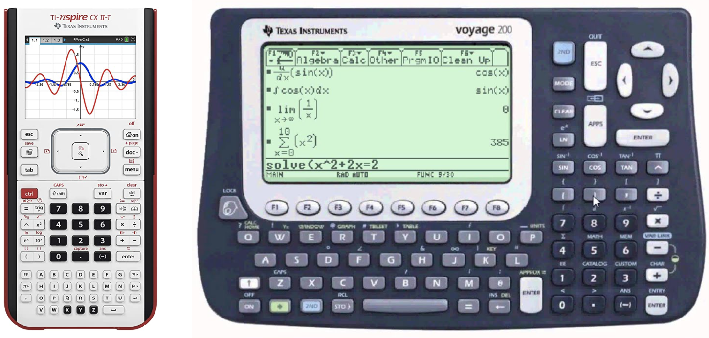
As humans, we use symbols to carry out computations analytically. This can also be realized on computers using symbolic computation. There are many so-called computer algebra systems (CAS) out there and you might already be familiar with one from school if you have used a graphing calculator there like the ones shown below.
But of course CAS is not limited to external devices but also available as software for normal computers. The most commonly used computer algebra systems are Mathematica and SageMath/SymPy. We will use Sympy in this course because it is open-source and a Python library compared to Mathematica. SageMath is based on Sympy and offers a number of additional functionalities, which we do not need in this class.
To illustrate the difference between numerical and symbolic computations,
we compare the output of the square root functions from numpy and sympy.
The code
import numpy as np
print(np.sqrt(8))
produces 2.8284271247461903 as output, which is an approximation to the
true value of (\sqrt{8}), while
import sympy as sp
print(sp.sqrt(8))
produces 2*sqrt(2), which is exact.
Basic Operations
We strongly advise you to try out the following small code examples yourself, preferably in a Jupyter notebook. There you can easily see the value of the variables and the equations can be rendered as latex. Just write the SymPy variable at the end of Jupyter cell without calling the
Defining Variables
Before solving any problem, we start defining our symbolic variables.
SymPy provides the constructor sp.Symbol() for this:
x = sp.Symbol('x')
This defines the Python variable x as a SymPy Symbol with the representation
'x'. If you print the variable in a Jupyter cell, you should see a rendered
symbol like: \( x \).
Since it might be annoying to define a lot variables, SymPy provides a another
function, which can initialize a arbitrary number of symbols.
x, y, t, omega = sp.symbols('x y t omega')
which is just a shorthand for
x, y, t, omega = [sp.Symbol(n) for n in ('x', 'y', 't', 'omega')]
Note that it is important to separate each symbol in the sp.symbols() call
with a space.
SymPy also provides often used symbols (Latin and Greek letters) as predefined
variables. They are located in the submodule called abc
and can be imported by calling
from sympy.abc import x, y, nu
Expressions
Now we can use these variables to define an expression. We first want to define the following expression: $$ x + 2 y $$ SymPy allows us to write this expression in Python as we would do on paper:
x, y = sp.symbols('x y')
f = x + 2 * y
If you now print f in Jupyter cell you should see the same rendered equation
as above.
Lets assume we want to multiply our expression not by \( x \). We can
just do the following:
g = x * f
Now, we can print g and should get:
$$
x (x + 2y)
$$
One may expect this expression to transform into
\(x^2 + 2xy\), but we get the factorized form instead. SymPy
only performs obvious simplifications automatically, since one might
prefer the expanded or the factorized form depending on the circumstances.
But we can easily switch between both representations using the
transformation functions expand and factor:
g_expanded = sp.expand(g)
If you print g_expanded, you should see the expanded form of the equation:
$$
x^2 + 2xy
$$
Factorization of g_expanded brings us back to where we started.
g_factorized = sp.factor(g_expanded)
with the following representation: $$ x (x + 2y) $$
If you prefer a more automated approach, you can use the function simplify.
SymPy will then try to figure out which form would be the most suitable.
We can also write more complicated functions using elementary functions:
t, omega = sp.symbols('t omega')
f = sp.sqrt(2) / sp.sympify(2) * sp.exp(-t) * sp.cos(omega*t)
Note that since the division operator / on a number produces
floating-point numbers, we should modify numbers with the function sympify.
When dealing with rationals like 2/5, we can use sp.Rational(2, 5) instead.
If you print f the rendered equation should look like:
$$
\frac{\sqrt{2} e^{-t} \cos \left( \omega t \right)}{2}
$$
On some platforms, you may get a nicely rendered expression. While other
platforms does not support LaTeX-rendering, you could try to turn on
unicode support by executing
sp.init_printing(use_unicode=True)
at the beginning of your code.
We can also turn our expression into a function with either one
f_func1 = sp.Lambda(t, f)
or multiple arguments
f_func2 = sp.Lambda((t, omega), f)
by using the Lambda function. In the first case printing of f_func1
should look like
$$
\left(t \mapsto \frac{\sqrt{2} e^{-t} \cos (\omega t)}{2}\right)
$$
while f_func2 should give you:
$$
\left((t, \omega) \mapsto \frac{\sqrt{2} e^{-t} \cos (\omega t)}{2}\right)
$$
As you can see, these are still symbolic expressions. But the Python object is
now a callable function with either one or two positional arguments.
This allows us to substitute e.g. the variable \( t \) with
a number:
f_func1(1)
This gives us: $$ \frac{\sqrt{2} \cos (\omega)}{2 e} $$ We can also call our second function, which takes 2 arguments (\(t\), and \(\omega\)).
f_func2(sp.Rational(1, 2), 1)
Which will result in:
$$
\frac{\sqrt{2} \cos \left(\frac{1}{2}\right)}{2 e^{\frac{1}{2}}}
$$
Note: We have now eliminated all variables and are left with an exact number, but this still
a SymPy object. You might wonder how we can transform this to a numerical value which
can be use by other Python modules. SymPy provides this transformation with the function
lambdify, this looks similar to the Lambda function and also returns a Python function, that
we can call. However, the returned value of this function is now numerical value.
import math
f_num = sp.lambdify((t, omega), f)
assert math.isclose(f_num(0, 1), math.sqrt(2)/2)

f_01_expr = f.subs([(t, 0), (omega, 1)])
f_01_expr_num = float(f_01_expr)
assert math.isclose(f_01_expr_num, math.sqrt(2)/2)

f_01_expr = f.subs([(t, 0), (omega, 1)])
f_01_expr_num = f_01_expr.evalf()
f_01_expr_num2 = f_01_expr.evalf(50)
Alternatively, we can convert the expression directly into a float
(or complex) by using the built-in functions float() or complex:
f_01_expr = f.subs([(t, 0), (omega, 1)])
f_01_expr_num = float(f_01_expr)
assert math.isclose(f_01_expr_num, math.sqrt(2)/2)
SymPy also offers us a way to convert an expression to a float (or complex):
f_01_expr = f.subs([(t, 0), (omega, 1)])
f_01_expr_num = f_01_expr.evalf()
f_01_expr_num2 = f_01_expr.evalf(50)
Although f_01_expr_num gives us the same result as the python float in the
first glance, its type is not ´float´, but rather sympy.core.numbers.Float.
Note the capital F. This is a floating point data type from sympy, which has
arbitrary precision. The last line, for example, evaluates the expression
with 50 valid decimal places instead of the standard 15 or 16 of Python's
built-in float.
Calculus
Calculus is hard. So why not let the computer do it for us?
Limits
Let us start by
evaluating the limit
$$\lim_{x\to 0} \frac{\sin(x)}{x}$$
We first define our variable \( x \) and the expression inside on the
right hand side. Then we can use the method limit to evaluate the
limit for \( x \to 0 \).
x = sp.symbols('x')
f = sp.sin(x) / x
lim = sp.limit(f, x, 0)
assert lim == sp.sympify(1)
Even one-sided limits like $$ \lim_{x\to 0^+} \frac{1}{x} \mathrm{\ \ vs.\ } \lim_{x\to 0^-} \frac{1}{x} $$ can be evaluated.
f = sp.sympify(1) / x
rlim = sp.limit(f, x, 0, '+')
assert rlim == sp.oo

llim = sp.limit(f, x, 0, '-')
assert llim == -sp.oo
Derivatives
Suppose we want find the first derivative of the following function
$$f(x, y) = x^3 + y^3 + \cos(x \cdot y) + \exp(x^2 + y^2)$$
We first start by defining the expression on the right side. In the next
step we can call the diff function, which expects an expression as the
first argument. The second to last argument (you can use one or more)
are the symbolic variables by which the expression will be differentiated.
x, y = sp.symbols('x y')
f = x**3 + y**3 + sp.cos(x * y) + sp.exp(x**2 + y**2)
f1 = sp.diff(f, x)
In this we create the first derivative of \( f(x, y) \) with respect to \(x\). You should get: $$ x^{3}+y^{3}+e^{x^{2}+y^{2}}+\cos (x y) $$
We can also build the second and third derivative with respect to x:
f2 = sp.diff(f, x, x)
f3 = sp.diff(f, (x, 3))
Note that two different methods for computing higher derivatives are presented here.
Of course it is also possible to create the first derivative with respect to \( x\) and \(y\):
f4 = sp.diff(f, x, y)
Evaluating Derivatives (or any other expression)
Sometimes, we want to evaluate derivatives, or just any expression at
specified points. For this purpose, we could again use Lambda to convert
the expression into a function and inserting values by function calls;
However, SymPy expressions have the subs method to avoid the detour:
f = x**3 + y**3 + sp.cos(x*y) + sp.exp(x**2 + y**2)
f3 = sp.diff(f, (x, 3))
g = f3.subs(y, 0)
h = f3.subs(y, x)
i = f3.subs(y, sp.exp(x))
j = f3.subs([(x, 1), (y, 0)])
This method takes a pair of arguments. The first one is the variable to be substituted and the second one the value. Note that the value can also be a variable or an expression. A list of such pairs can also be supplied to substitute multiple variables.
Integrals
Even the most challenging part in calculus (integrals) can be evaluated $$ \int \mathrm{e}^{-x} \mathrm{d}x $$
f = sp.exp(-x)
f_int = sp.integrate(f, x)
This evaluates to $$ -e^{-x} $$ Note that SymPy does not include the constant of integration. But this can be added easily by oneself if needed.
A definite integral could be computed by substituting the integration variable
with upper and lower bounds using subs. But it is more straightforward to
just pass the tuple with both bounds as the second argument to the
integrate function:
Suppose we want to compute the definite integral
$$\int_{0}^{\infty} \mathrm{e}^{-x}\ \mathrm{d}x$$
one can write
f = sp.exp(-x)
f_dint = sp.integrate(f, (x, 0, sp.oo))
assert f_dint == sp.sympify(1)
which evaluates to 1.
Also multivariable integrals like $$ \int_{-\infty}^{\infty} \int_{-\infty}^{\infty} \mathrm{e}^{-x^2-y^2}\ \mathrm{d}x \mathrm{d}y $$ can be easily solved. In this case the integral
f = sp.exp(-x**2 - y**2)
f_dint = sp.integrate(f, (x, -sp.oo, sp.oo), (y, -sp.oo, sp.oo))
assert f_dint == sp.pi
evaluates to \( \pi \).
Application: Hydrogen Atom
We learned in the bachelor quantum mechanics class that the wavefunction of the hydrogen atom has the following form: $$ \psi_{nlm}(\mathbf{r})=\psi(r, \theta, \phi)=R_{n l}(r) Y_{l m}(\theta, \phi) $$ where \(R_{n l}(r) \) is the radial function and \(Y_{l m}\) are the spherical harmonics. The radial functions are given by $$ R_{n l}(r)=\sqrt{\left(\frac{2}{n a}\right)^{3} \frac{(n-l-1) !}{2 n[(n+l) !]}} e^{-r / n a}\left(\frac{2 r}{n a}\right)^{l}\left[L_{n-l-1}^{2 l+1}(2 r / n a)\right] $$ Here \(n, l\) are the principal and azimuthal quantum number. The Bohr radius is denoted by \( a\) and \( L_{n-l-1}^{2l+1} \) is the associated/generalized Laguerre polynomial of degree \( n - l -1\). We will work with atomic units in the following, so that \( a = 1\). With this we start by defining the radial function:
def radial(n, l, r):
    n, l, r = sp.sympify(n), sp.sympify(l), sp.sympify(r)
    n_r = n - l - 1
    r0 = sp.sympify(2) * r / n
    c0 = (sp.sympify(2)/(n))**3
    c1 = sp.factorial(n_r) / (sp.sympify(2) * n * sp.factorial(n + l))
    c = sp.sqrt(c0 * c1)
    lag = sp.assoc_laguerre(n_r, 2 * l + 1, r0)
    return c * r0**l * lag * sp.exp(-r0/2)
We can check if we have any typo in this function by simply calling it with the three symbols
n, l, r = sp.symbols('n l r')
radial(n, l, r)
In the next step we can define the wave function by building the product of the radial function and the spherical harmonics.
from sympy.functions.special.spherical_harmonics import Ynm

def wavefunction(n, l, m, r, theta, phi):
    return radial(n, l, r) * Ynm(l, m, theta, phi).expand(func=True)
With this in hand, we have everything we need and we can start playing with wave functions of the Hydrogen atom. Let us begin with the simplest one, the 1s function \( \psi_{100} \).
n, l, m, r, theta, phi = sp.symbols('n l m r theta phi')
psi_100 = wavefunction(1, 0, 0, r, theta, phi)
We can now use what we learned in the previous chapter and evaluate for example the wavefunction in the limit of \(\infty\) $$ \lim_{r\to \infty} \psi_{100}(r, \theta, \phi) $$
psi_100_to_infty = sp.limit(psi_100, r, sp.oo)
assert psi_100_to_infty == sp.sympify(0)
This evaluates to zero, as we would expect. Now let's check if our normalization of the wave function is correct. For this we expect, that the following holds: $$ \int_{0}^{+\infty} \mathrm{d}r \int_{0}^{\pi} \mathrm{d}\theta \int_{0}^{2\pi} \mathrm{d}\phi \ r^2 \sin(\theta)\ \left| \psi_{100}(r,\theta,\phi) \right|^2 = 1 $$ We can easily check this, since we already learned how to calculate definite integrals.
dr = (r, 0, sp.oo)
dtheta = (theta, 0, sp.pi)
dphi = (phi, 0, 2*sp.pi)
norm = sp.integrate(r**2 * sp.sin(theta) * sp.Abs(psi_100)**2, dr, dtheta, dphi)
assert norm == sp.sympify(1)
Visualizing the wave functions of the H atom.
To visualize the wave functions we need to evaluate them on a finite grid.
Radial part of wave function.
For this example we will examine the radial part of the first 4 s-functions. We start by defining them:
r = sp.symbols('r')
r10 = sp.lambdify(r, radial(1, 0, r))
r20 = sp.lambdify(r, radial(2, 0, r))
r30 = sp.lambdify(r, radial(3, 0, r))
r40 = sp.lambdify(r, radial(4, 0, r))
This gives us 4 functions that will return numeric values of the radial part at some radius \(r\). The radial electron probability is given by \(r^2 |R(r)|^2\). We will use these functions to evaluate the wave functions on a grid and plot the values with Matplotlib.
import matplotlib.pyplot as plt

r0 = 0
r1 = 35
N = 1000
r_values = np.linspace(r0, r1, N)
fig, ax = plt.subplots(1, 1, figsize=(8, 5))
ax.plot(r_values, r_values**2*r10(r_values)**2, color="black", label="1s")
ax.plot(r_values, r_values**2*r20(r_values)**2, color="red", label="2s")
ax.plot(r_values, r_values**2*r30(r_values)**2, color="blue", label="3s")
ax.plot(r_values, r_values**2*r40(r_values)**2, color="green", label="4s")
ax.set_xlim([r0, r1])
ax.legend()
ax.set_xlabel(r"distance from nucleus ($r/a_0$)")
ax.set_ylabel(r"electron probability ($r^2 |R(r)|^2$)")
fig.show()

Spherical Harmonics
In the next step, we want to graph the spherical harmonics. To do
this, we first import all the necessary modules and then define first the
symbolic spherical harmoncis, Ylm_sym, and then the numerical function Ylm.
from sympy.functions.special.spherical_harmonics import Ynm
import sympy as sp
import numpy as np
import matplotlib.pyplot as plt
from matplotlib import cm
%config InlineBackend.figure_formats = ['svg']

l, m, theta, phi = sp.symbols("l m theta phi")
Ylm_sym = Ynm(l, m, theta, phi).expand(func=True)

Ylm = sp.lambdify((l, m, theta, phi), Ylm_sym)
The variable Ylm now contains a Python function with 4 arguments (l, m,
theta, phi) and returns the numeric value (complex number, type: complex)
of the spherical harmonics. To be able to display the function graphically,
however, we have to evaluate the function not only at one point, but on a
two-dimensional grid (\(\theta, \phi\)) and then display the values on this
grid. Therefore, we define the grid for \(\theta\) and \(\phi\) and evaluate
the \(Y_{lm} \) for each point on this grid.
N = 1000
theta = np.linspace(0, np.pi, N)
phi = np.linspace(0, 2*np.pi, N)
theta, phi = np.meshgrid(theta, phi)
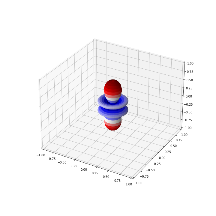
l = 3
m = 0
Ylm_num = 1/2 * np.abs(
Ylm(l, m, theta, phi) + np.conjugate(Ylm(l, m, theta, phi))
)
Now, however, we still have a small problem because we want to represent our data points in a Cartesian coordinate system, but our grid points are defined in spherical coordinates. Therefore it is necessary to transform the calculated values of Ylm into the Cartesian coordinate system. The transformation reads:
x = np.cos(phi) * np.sin(theta) * Ylm_num
y = np.sin(phi) * np.sin(theta) * Ylm_num
z = np.cos(theta) * Ylm_num
Now we have everything we need to represent the spherical harmonics in 3
dimensions. We do a little trick and map the data points to a number range from
0 to 1 and store these values in the variable colors. This allows us to
color the spherical harmonics with a colormap
from Matplotlib.
colors = Ylm_num / (Ylm_num.max() - Ylm_num.min())

fig = plt.figure(figsize=(10, 10))
ax = fig.add_subplot(111, projection="3d")

ax.plot_surface(x, y, z, facecolors=cm.seismic(colors))

ax.set_xlim([-1, 1])
ax.set_ylim([-1, 1])
ax.set_zlim([-1, 1])
fig.show()
For the above example with \( Y_{30}\), the graph should look like
Application: Harmonic Oscillator
The quantum harmonic oscillator is described by the wavefunctions $$ \psi_{n}(x) = \frac{1}{\sqrt{2^n n!}} \left( \frac{m \omega}{\pi \hbar} \right)^{1/4} \exp\left(-\frac{m\omega x^2}{2\hbar}\right) H_{n}\left( \sqrt{\frac{m\omega}{\hbar}} x \right) $$ where the functions \(H_{n}(z)\) are the physicists' Hermite polynomials: $$ H_{n}(z) = (-1)^n\ \mathrm{e}^{z^2} \frac{\mathrm{d}^n}{\mathrm{d}z^n} \left( \mathrm{e}^{-z^2} \right) $$ The corresponding energy levels are $$ E_{n} = \hbar \omega \left( n + \frac{1}{2} \right) $$
We now want to use SymPy to compute eigenenergies and eigenfunctions.
We start by importing sympy and necessary variables:
import sympy as sp
from sympy.abc import x, m, omega, n, z
The eigenenergies are straightforward to compute. One can just use the definition directly and substitute \(n\) with an integer, e.g. 5:
def energy(n):
    e = omega * (n + sp.Rational(1, 2))
    return e

e_5 = energy(5)
This outputs \(\frac{11}{2}\). Note that atomic units are used for simplicity.
In order to evaluate the wave function, we have to at first compute the Hermite polynomial. There are multiple ways to do it. The first is to use its definition directly and compute higher order derivatives of the exponential function:
def hermite_direct(n):
    h_n = (-1)**n * sp.exp(z**2) * sp.diff(sp.exp(-z**2), (z, n))
    h_n = sp.simplify(h_n)
    return h_n
Alternatively, we could use recurrence relation for Hermite polynomials. This will be left as an exercise for the course attendees.
For n = 5, we obtain the polynomial
$$ H_5(x) = 32 x^5 - 160 x^3 + 120 x$$
We can then use this to evaluate the wave function:
def wfn(n):
    nf = (1/sp.sqrt(2**n * sp.factorial(n))) \
         * ((m*omega)/sp.pi)**sp.Rational(1, 4)
    expf = sp.exp(-(m*omega*x**2)/2)
    hp = hermite_direct(n).subs(z, sp.sqrt(m*omega)*x)
    psi_n = sp.simplify(nf * expf * hp)

    return psi_n

psi_5 = wfn(5)
For a system with, say, \(m = 1\) and \(\omega = 1\), we can construct its wave function by
psi_5_param = psi_5.subs([(m, 1), (omega, 1)])
Further substituting x with any numerical value would evaluate the
wave function at that point.
We can again convert the sympy expression to a numpy function and plot some wavefunctions.
import numpy as np
import matplotlib.pyplot as plt

x_values = np.linspace(-5, 5, 100)

fig, ax = plt.subplots(1, 1, figsize=(8, 5))
ax.set_xlabel('$x$')

ax.plot(x_values, 0.5 * x_values**2, c='k', lw=2)
for i in range(5):
    psi_param = wfn(i).subs([(m, 1), (omega, 1)])
    psi_numpy = sp.lambdify(x, psi_param)
    ax.plot(x_values, psi_numpy(x_values) + (0.5 + i), label=f'n = {i}')

ax.set_xlim(-4, 4)
ax.set_ylim(-0.1, 6.1)
ax.legend()

plt.show()
This code block produces

Sometimes one might just want to use SymPy to generate symbolic expressions
to be used in functions. Instead of typing the results in by hand, one could
use one of SymPy's built-in printers. Here, we shall use NumPyPrinter,
which converts a SymPy expression to a string of python code:
from sympy.printing.numpy import NumPyPrinter
printer = NumPyPrinter()
code = printer.doprint(psi_5_param)
code = code.replace('numpy', 'np')
print(code)
This output can be copied and used to evaluate \(\psi_{5}(x)\).
Since we often import NumPy with the alias np, numpy from the original
string is replaced.
Molecular Integrals
In quantum chemistry, the very well known Hartree-Fock (HF) method is used to approximate the ground-state electronic structure of a molecule. The method involves solving the HF equation, which is given by $$ \hat{f} | \varphi_i \rangle = \epsilon_i | \varphi_i \rangle $$ where \(\hat{f}\) is the Fock operator, \(| \varphi_i \rangle \) is the \(i\)-th eigenfunction, \(\epsilon_i\) is the corresponding eigenvalue. We identify the eigenfunction with canonical molecular orbitals and the eigenvalues with orbital energies.
The Fock operator is defined as $$ \hat{f} = \hat{h}^{\mathrm{core}} + \sum_{j=1}^{N} \left( \hat{J}_j - \hat{K}_j \right) $$ with the one-electron Hamiltonian \(\hat{h}^{\mathrm{core}}\), the Coulomb operator \(\hat{J}_j\) and the exchange operator \(\hat{K}_j\), and \(N\) stands for the number of electrons.
Since \(\hat{h}^{\mathrm{core}}\) contains differential operators and \(\hat{J}_j\) and \(\hat{K}_j\) have integrals in them, the HF equation is an integro-differential equation, for which a closed-form solution is extremly difficult to obtain and analytical solutions are only known for the simplest cases.
Therefore, we utilize numerical methods to solve the HF equation. Though popular in other fields, a discretization is very impractical hier. Considering the rapid change of electronic density from nuclei to bonds and bond lengths of roughly 1 Å, at least 4 points per Å should be used for a crude representation of the wavefunction. Also, we should add a boundary to properly describe the fall-off of the wavefunction. For a medium-sized molecule, e.g. porphin, which is around 10 Å across, a box of the dimension 15 Å × 15 Å × 5 Å would be appropriate, which translates to 60 × 60 × 20 = 72000 grid points. This is far from practical. If we wish a finer granulated grid, or calculations for larger molecules, discretization will become infeasible rather quickly.
So, the spatial grid is a very inefficient basis for the HF equation. Because the molecule consists of atoms, it should be possible to represent the molecular orbitals with some sort of combinations of atomic orbitals. The simplest combination is the linear combination. In this case, our basis are atom-centered wavefunctions \(\chi_\mu\), and the molecular orbitals can be expressed as $$ | \varphi_i \rangle = \sum_{\mu} c_{\mu i} \chi_\mu $$ where \(\mu\) indexes the atomic basis functions.
Inserting this Ansatz into the HF equation and projecting both sides onto \(\langle \chi_\nu|\), we obtain $$ \begin{align} \langle \chi_\nu | \hat{f} | \sum_{\mu} c_{\mu i} \chi_\mu \rangle &= \epsilon_i \langle \chi_\nu | \sum_{\mu} c_{\mu i} \chi_\mu \rangle \\ \sum_{\mu} \langle \chi_\nu | \hat{f} | \chi_\mu \rangle c_{\mu i} &= \sum_{\mu} \langle \chi_\nu | \chi_\mu \rangle c_{\mu i} \epsilon_i \\ \mathbf{F}\vec{c}_i &= \mathbf{S}\vec{c}_i\epsilon_i \end{align} $$ where \(\mathbf{F}\) is the Fock matrix, \(\vec{c}_i\) is the coefficient vector of the \(i\)-th molecular orbital, \(\mathbf{S}\) is the overlap matrix, and \(\epsilon_i\) is the energy of the \(i\)-th molecular orbital.
The new equation is called Roothaan-Hall equation, where the difficult derivatives and integrals of the unknown molecular orbitals is reduced to derivatives and integrals of known basis functions. After evaluating these integrals in \(\mathbf{F}\) and \(\mathbf{S}\), the actual solving step is easily done using some linear algebra.
A closer inspection of the matrices \(\mathbf{F}\) and \(\mathbf{S}\) reveals that four types of molecular integrals exist:
- Overlap integrals: \(\langle \chi_\mu | \chi_\nu \rangle\)
- Kinetic energy integrals: \(\langle \chi_\mu | -\frac{1}{2} \nabla^2 | \chi_\nu \rangle\)
- nuclear attraction integrals: \(\langle \chi_\mu | -Z_{\mathrm{nuc}}/R_{\mathrm{nuc}} | \chi_\nu \rangle\)
- electron repulsion integrals: \(\langle \mu \nu | \lambda \sigma \rangle\)
In this chapter, some basis concepts of basis functions will be introduced, followed by symbolic calculation of closed-form expressions for molecular integrals. In the end, we will use these expressions to generate a module, which performs all these integrals.
Gaussian Type Orbitals
The Schrödinger equation of the hydrogen atom can be solved analytically and the obtained wave functions have the radial part $$ R_{nl}(r) = N_{nl} \left[ L_{n-l-1}^{2l+1} \left( \frac{2r}{na} \right) \right] \left( \frac{2 r}{n a} \right)^l \exp\left(-\frac{r}{na}\right) $$ where \(n\), \(l\) are the principal and azimuthal quantum number, respectively, \(N_{nl}\) is the normalisation constant, \(L_{n-l-1}^{2l+1}\) is the associated Laguerre polynomial and \(a\) stands for Bohr radius.
Ignoring the normalisation constant and the polynomial factor, the wavefunction boils down to \(\exp(-\zeta r)\). One may assume that all atomic orbitals have this general form, the so-called Slater type orbitals (STO). These orbitals have a cusp in the origin, which accurately describes the electron distribution at nuclei.
STOs, however, are not very easy to integrate. Analytically expressions of one-electron integrals involving STOs can be obtained, though they are rather cumbersome. Two-electron integrals involving STOs cannot be solved analytically, so ei)ther numerical integration or approximations must be applied. This make the use of STOs in quantum chemistry very impractical.
Instead, the Gaussian type orbitals (GTO), which has the general form \(\exp(-\alpha r^2)\), is widely used for quantum chemistry. Although it does not accurately represents the correct electronic density at nuclei, relatively simple analytical expressions for molecular integrals involving GTOs, including two-electron integrals, exist, even for two-electron integrals
Cartesian Gaussian Orbitals
The most intuitive form of GTOs is the Cartesian form, which is expressed as $$ g_{nl}(\vec{r};\alpha, \vec{A}) = N_{nl}(\alpha)\ \|\vec{r} - \vec{A}\|^{n-l-1} \ (x-A_x)^{l_x} (y-A_y)^{l_y} (z-A_z)^{l_z} \ \mathrm{e}^{-\alpha \| \vec{r}-\vec{A} \|^2} $$ with the nucleus sitting at \(\vec{A}\) and \(l_x + l_y + l_z = l\). Some examples values of \(l\) and the corresponding atomic orbitals are shown in the following table:
| \(l_x\) | \(l_y\) | \(l_z\) | Orbital |
|---|---|---|---|
| 0 | 0 | 0 | \(s\) |
| 1 | 0 | 0 | \(p_x\) |
| 0 | 1 | 0 | \(p_y\) |
| 0 | 0 | 1 | \(p_z\) |
| 1 | 1 | 0 | \(d_{xy}\) |
| 1 | 0 | 1 | \(d_{xz}\) |
| 0 | 1 | 1 | \(d_{yz}\) |
| 2 | 0 | 0 | \(d_{x^2}\) |
| 0 | 2 | 0 | \(d_{y^2}\) |
| 0 | 0 | 2 | \(d_{z^2}\) |
Gaussian Product Theorem
The existence of relatively simple expressions molecular integrals involving GTOs is partly due to the Gaussian product theorem, which states that the product between two 1s Gaussians (\(n=0\), \(l_x = l_y = l_z = 0\)) is another 1s Gaussian. We shall demonstrate this theorem for two (unnormalized) 1D-Gaussians $$ \begin{align} g(x;\alpha,A_x) &= \exp\left(-\alpha ( x - A_x )^2 \right) \\ &\text{and} \\ g(x;\beta,B_x) &= \exp\left(-\beta ( x - B_x )^2 \right) \end{align} $$
By taking the product of the two Gaussian functions, we obtain
$$ g(x;\alpha,A_x) \cdot g(x;\beta,B_x) = \exp\left(-\alpha ( x - A_x )^2\right) \cdot \exp\left(-\beta ( x - B_x )^2\right) $$
We can simplify this expression by using the properties of exponents:
$$ \begin{align} g(x;\alpha,A_x) \cdot g(x;\beta,B_x) &= \exp\left(-\alpha ( x^2 - 2A_x x + A_x^2 )\right) \cdot \exp\left(-\beta ( x^2 - 2B_x x + B_x^2 )\right) \\ &= \exp\left(-\alpha x^2 + 2\alpha A_x x - \alpha A_x^2 \right) \cdot \exp\left(-\beta x^2 + 2\beta B_x x - \beta B_x^2 \right) \\ &= \exp\left(-(\alpha + \beta)x^2 + 2(\alpha A_x + \beta B_x)x - (\alpha A_x^2 + \beta B_x^2)\right) \\ &= \exp\left(-( \alpha + \beta) \left(x^2 - 2\dfrac{\alpha A_x + \beta B_x}{\alpha + \beta} x + \dfrac{\alpha^2 A_x^2 + \beta^2 B_x^2}{(\alpha + \beta)^2} - \dfrac{\alpha B_x^2 + \beta A_x^2}{\alpha + \beta} \right)\right) \\ &= \exp\left(-( \alpha + \beta) \left(x - \dfrac{\alpha A_x + \beta B_x}{\alpha + \beta}\right)^2 - \dfrac{\alpha\beta}{\alpha + \beta}(A_x - B_x)^2 \right) \end{align} $$
In the last step, we completed the square inside the exponent to obtain a Gaussian function. By defining $$ \begin{align} p &= \alpha + \beta \\ \mu &= \frac{\alpha \beta}{\alpha + \beta} \\ X_{AB} &= A_x - B_x \\ P_x &= \frac{\alpha A_x + \beta B_x}{\alpha + \beta} \end{align} $$ we obtain $$ g(x;\alpha,A_x) \cdot g(x;\beta,B_x) = g(x;p,P_x) \exp\left( -\mu X_{AB}^2 \right) $$ a new Gaussian at the "center of mass" \(P_x\) with the total exponent \(p\), scaled by \(\exp\left( \mu X_{AB}^2 \right)\). Since Gaussian orbitals can be easily factored into Cartesian directions, a proof for 3D-Gaussians follow trivially from the proof for 1D-Gaussians.
Contracted Gaussians
Because Gaussians do differ quite a bit from Slater functions, we can make them more accurate by using a linear comination of Gaussians, i.e. $$ G(x; {\alpha_i}, {c_i}, \vec{A}) = \sum_{i=1}^N c_i g(\vec{x}; \alpha_i, \vec{A}) $$ where \(G(x; {\alpha_i}, {c_i}, \vec{A})\) is called a contracted Gaussian. To avoid confusion, we shall call \(g(\vec{x}; \alpha_i, \vec{A})\) primitive Gaussian.
Apart from being more accurate, another advantage of using contracted Gaussian is the exclusive use of orbitals without radial nodes. In other words, we only need Gaussians of the form $$ g_{l}(\vec{r};\alpha, \vec{A}) = N_{l}(\alpha)\ (x-A_x)^{l_x} (y-A_y)^{l_y} (z-A_z)^{l_z} \ \mathrm{e}^{-\alpha \| \vec{r}-\vec{A} \|^2} $$ Note that the factor \(\|\vec{r} - \vec{A}\|^{n-l-1}\) is gone and the orbital no longer depends on the principal quantum number \(n\). Because we can now omit the index \(n\) on \(g\), we can use \(i\), \(j\) and \(k\) instead of the verbose \(l_x\), \(l_y\) and \(l_z\), which are difficult to read when written as exponents. Such Cartesian Gaussians can thus be written as $$ g_{ijk}(\vec{r};\alpha, \vec{A}) = N_{l}(\alpha)\ (x-A_x)^{i} (y-A_y)^{j} (z-A_z)^{k} \ \mathrm{e}^{-\alpha \| \vec{r}-\vec{A} \|^2} $$
This simplification can be done out of two reasons: On the one hand, the radial nodes are located in the neighborhood of core orbitals, which do not contribute much to chemical bonding. On the other hand, a linear combination of primitive Gaussians with some negative contraction coefficients can approximate an atomic orbital with nodes.
We shall now take a look at an example of Gaussian basis sets:
#BASIS SET: (6s,3p) -> [2s,1p]
C    S
      0.7161683735E+02       0.1543289673E+00
      0.1304509632E+02       0.5353281423E+00
      0.3530512160E+01       0.4446345422E+00
C    SP
      0.2941249355E+01      -0.9996722919E-01       0.1559162750E+00
      0.6834830964E+00       0.3995128261E+00       0.6076837186E+00
      0.2222899159E+00       0.7001154689E+00       0.3919573931E+00
This is the STO-3G basis set for the carbon atom. The first line with the
notation (6s,3p) -> [2s,1p] tells us that this basis set consists of
6 primitive Gaussian functions of the s-type and 3 primitive Gaussian
functions of the p-type. These primitive functions are then contracted
to form 2 s-type and 1 p-type contracted Gaussian functions.
The rest of this snippet contains two blocks, with every block starting with a line clarifying the atom and orbital type. The other lines have either two or three columns. The first block describes an s-type basis function with the exponents listed in the first column and the contraction coefficients listed in the second column. The second block describes an s-type and a p-type basis function with the same orbital exponents listed in the first column. The next two columns contain the contraction coefficients for s-orbitals and p-orbitals, respectively.
Note: The contraction coefficients do NOT include the normalization constants for the primitive Gaussians. So you have to include it when constructing contracted Gaussians.
Hermite Gaussian Orbitals
Though very intuitive, the Cartesian Gaussians are not easy to integrate except for s-type Gaussians, since the polynomial product makes the evaluation quite tedious. It would be nice if we could somehow generate integrals involving higher orbital angular momenta from integrals involving only s-type Gaussians.
Hermite Gaussian Functions
We now introduce another form of GTOs, the Hermite Gaussians. Ignoring the normalisation constant, they are defined as
$$ h_{ijk}(\vec{r}; \alpha, \vec{A}) = \left( \frac{\partial}{\partial A_x} \right)^{i} \left( \frac{\partial}{\partial A_y} \right)^{j} \left( \frac{\partial}{\partial A_z} \right)^{k} \mathrm{e}^{-\alpha \| \vec{r} - \vec{A} \|^2} $$
Although it might look very complicated in the first glance, it is essentially a Cartesian Gaussian with the Cartesian polynomial part replaced by a polynomial obtained through differentiation of an s-type Gaussian, or the Hermite polynomial.
Just like their Cartisian counterparts, the Hermite Gaussians can also be factored into Cartesian directions. A 1D Hermite Gaussian of degree \(k\) can thus be expressed as $$ h_{k}(x; \alpha, A_x) = \left( \frac{\partial}{\partial A_x} \right)^k \mathrm{e}^{-\alpha ( x - A_x )^2} $$
Recurrence Relations
While it is straight-forward to generate a Cartesian Gaussian of degree \(n + 1\) from a degree \(n\) one by just multiplying \(x - A_x\) to it, i.e. $$ g_{n + 1}(x) = (x - A_x)\ g_{n}(x) $$ the relation for Hermite Gaussians is a bit complicated.
We shall start with the definition of Hermite Gaussians, which states $$ h_{k+1}(x) = \left( \frac{\partial}{\partial A_x} \right)^k \frac{\partial}{\partial A_x} \exp\left( -\alpha (x - A_x)^2 \right) = 2 \alpha \left( \frac{\partial}{\partial A_x} \right)^k (x - A_x) \ \mathrm{e}^{-\alpha (x - A_x)^2} $$ The \(k\)-th derivative of the product \( (x - A_x) \cdot \mathrm{e}^{-\alpha (x - A_x)^2} \) can be calculated using the general Leibniz rule: $$ \left(\frac{\partial}{\partial A_x}\right)^k \left[(x - A_x) \mathrm{e}^{-\alpha (x - A_x)^2}\right] = \sum_{j=0}^k \binom{k}{j} \left(\frac{\partial}{\partial A_x}\right)^j (x - A_x) \left(\frac{\partial}{\partial A_x}\right)^{k-j} \mathrm{e}^{-\alpha (x - A_x)^2} $$
Since the first factor \((x - A_x)\) is a first-order polynomial in \(A_x\), derivatives with order 2 or higher become zero. The whole expression thus simplifies to $$ \begin{align} \left(\frac{\partial}{\partial A_x}\right)^k \left[(x - A_x) \mathrm{e}^{-\alpha (x - A_x)^2}\right] &= \binom{k}{0} \left(\frac{\partial}{\partial A_x}\right)^0 (x - A_x) \left(\frac{\partial}{\partial A_x}\right)^{k} \mathrm{e}^{-\alpha (x - A_x)^2} \\ &\hphantom{=} + \binom{k}{1} \left(\frac{\partial}{\partial A_x}\right)^1 (x - A_x) \left(\frac{\partial}{\partial A_x}\right)^{k-1} \mathrm{e}^{-\alpha (x - A_x)^2} \\ &= (x - A_x) \left(\frac{\partial}{\partial A_x}\right)^{k} \mathrm{e}^{-\alpha (x - A_x)^2} - k \left(\frac{\partial}{\partial A_x}\right)^{k-1} \mathrm{e}^{-\alpha (x - A_x)^2} \\ &= (x - A_x)\ h_k(x) - k\ h_{k-1}(x) \end{align} $$ Combined with the equation for \(h_{k+1}(x)\) above, we get $$ h_{k+1}(x) = 2\alpha \left[ (x - A_x)\ h_k(x) - k\ h_{k-1}(x) \right] $$ We can thus get the Hermite Gaussian of order \(k+1\) with Hermite Gaussians of order \(k\) and \(k-1\). This kind of relations, where an object with one or several indices is related to objects with smaller indices, are called recurrence relations.
The recurrence relation for Hermite Gaussians is often expressed as $$(x - A_x) h_{k}(x) = \frac{1}{2 \alpha} h_{k+1}(x) + k h_{k-1}(x)$$ which is obtained by simple algebraic manupulation from the recurrence relation above.
Why are Hermite Gaussians useful? suppose we want to evaluate an integral involving a \(k\)-th order Hermite Gaussian, we can reduce it to an integral involving an zeroth order Hermite Gaussian as follows $$ \begin{align} \int h_k(x) f(x)\ \mathrm{d}x &= \int h_k(x)\ f(x)\ \mathrm{d}x \\ &= \int \left( \frac{\partial}{\partial A_x} \right)^k \mathrm{e}^{-\alpha (x - A_x)^2} f(x)\ \mathrm{d}x \\ &= \left( \frac{\partial}{\partial A_x} \right)^k \int \mathrm{e}^{-\alpha (x - A_x)^2} f(x)\ \mathrm{d}x \\ &= \left( \frac{\partial}{\partial A_x} \right)^k \int h_0(x)\ f(x)\ \mathrm{d}x \end{align} $$ where \(f(x)\) denotes an arbitrary function. Therefore, if we can solve an integral for \(h_0(x)\), we can solve the integrals for all \(h_k (x)\).
Hermite Gaussian Expansion
However, since our basis functions are Cartesian Gaussians, we have to expand them into Hermite Gaussians: $$ g_n(x) = \sum_k c_{kn} h_k(x) $$
To find the expansion coefficients, we shall examine \(g_{n+1}\): $$ \begin{align} g_{n+1} &= (x-A_x)\cdot g_n \\ &= (x-A_x) \cdot \sum_k c_{kn} h_k \\ &= \sum_k c_{kn} (x-A_x)\ h_k \\ &= \sum_k c_{kn} \left( \frac{1}{2\alpha} h_{k+1} + h_{k-1} \right) \\ &= \sum_k \frac{1}{2\alpha} c_{kn} h_{k+1} + \sum_k k c_{kn} h_{k-1} \end{align} $$ Note that we have used the recurrence relation for Hermite Gaussians in the second last step. Since the summation indices can be named as we like, we shall replace \(k\) with \(k+1\) in the first sum and with \(k-1\) in the second sum to obtain $$ g_{n+1} = \sum_k \frac{1}{2\alpha} c_{k-1,n} h_{k} + \sum_k (k+1) c_{k+1,n} h_{k} = \sum_k \left( \frac{1}{2\alpha} c_{k-1,n} + (k+1) c_{k+1,n} \right) h_k $$ By evaluating \(g_{n+1}\) directly, we obtain $$ g_{n+1} = \sum_k c_{k,n+1} h_k $$ Comparing the coefficients for each \(h_k\), we can get the recurrence relation for the expansion coefficients: $$ c_{k,n+1} = \frac{1}{2\alpha}\ c_{k-1,n} + (k+1)\ c_{k+1,n} $$
Such recurrence relations can be intuitively implemented in a recursive manner:
import sympy as sp
from functools import lru_cache


@lru_cache(maxsize=None)
def get_ckn(k, n, p):
    """
    Calculate the expansion coefficient C_{k,n} for a
    Cartesian Gaussian basis function with angular momentum n
    in terms of Hermite Gaussians of order k.

    The recursive formula used is:
    C_{k, n} = 1/(2 * p) * C_{k-1, n-1} + (k + 1) * C_{k+1, n-1}

    Args:
        k (int): Order of the Hermite Gaussian function.
        n (int): Angular momentum of the Cartesian Gaussian basis function.
        p (float): Exponent of the Gaussian functions.

    Returns:
        float: Expansion coefficient C_{k, n}.
    """
    if k == n == 0:
        return sp.sympify(1)
    elif (k == 0) and (n == 1):
        return sp.sympify(0)
    elif (k == 1) and (n == 1):
        return (1 / (2 * p))
    elif k > n:
        return sp.sympify(0)
    elif k < 0:
        return sp.sympify(0)
    else:
        return (1 / (2 * p)) * get_ckn(k - 1, n - 1, p) \
                + (k + 1) * get_ckn(k + 1, n - 1, p)
The function decorater lru_cache to speed up the execution.
Overlap Integrals
We can now proceed to calculate molecular integrals, starting with overlap integrals. An overlap integral between two centers \(A\) and \(B\) are defined as $$ S_{ijk,lmn}^{A,B} = \int g_{ijk}(\vec{r};\alpha, \vec{A}) \ g_{lmn}(\vec{r};\beta, \vec{B}) \ \mathrm{d}^3 r $$ Because Cartesian Gaussians are factorizable, we can calculate the overlap for each Cartesian direction, i.e., $$ S_{ijk,lmn}^{A,B} = S_{il}^{A_x, B_x}\ S_{jm}^{A_y, B_y}\ S_{kn}^{A_z, B_z} $$ Therefore, we only have to deal with overlaps between 1D Gaussians.
Hermite Gaussian Overlaps
We now examine the overlap between two (unnormalized) 1D Hermite Gaussian: $$ \begin{align} E_{k l}^{A_x, B_x} &= \int h_{k}(x;\alpha, A_x) \ h_{l}(x;\beta, B_x) \ \mathrm{d} x \\ &= \int \left( \frac{\partial}{\partial A_x} \right)^k \mathrm{e}^{-\alpha(x-A_x)^2} \left( \frac{\partial}{\partial B_x} \right)^l \mathrm{e}^{-\beta(x-B_x)^2} \mathrm{d} x \\ &= \left( \frac{\partial}{\partial A_x} \right)^k \left( \frac{\partial}{\partial B_x} \right)^l \int \mathrm{e}^{-\alpha(x-A_x)^2} \mathrm{e}^{-\beta(x-B_x)^2} \mathrm{d} x \\ &= \left( \frac{\partial}{\partial A_x} \right)^k \left( \frac{\partial}{\partial B_x} \right)^l E_{00}^{A_x,B_x} \end{align} $$ By using the Gaussian product theorem the integral \(E_{00}^{A_x,B_x}\) is reduced to $$ \begin{align} E_{00}^{A_x,B_x} &= \mathrm{e}^{-\mu X_{AB}^2} \int \mathrm{e}^{-p (x - P_x)^2} \\ &= \mathrm{e}^{-\mu X_{AB}^2} \sqrt{\frac{\pi}{p}} \end{align} $$ with $$ \begin{align} p &= \alpha + \beta \\ \mu &= \frac{\alpha \beta}{\alpha + \beta} \\ X_{AB} &= A_x - B_x \\ P &= \frac{\alpha A_x + \beta B_x}{\alpha + \beta} \end{align} $$ Substituting the variables back, we get $$ E_{00}^{A_x,B_x} = \sqrt{\frac{\pi}{\alpha + \beta}}\ \exp \left( -\frac{\alpha \beta}{\alpha + \beta} (A_x - B_x)^2 \right) $$ Differentiate this expression with respect to \(A_x\) and \(B_x\) will deliver us with all possible overlap integrals between Hermite Gaussians.
Cartesian Gaussian Overlaps
By expanding Cartesian Gaussians into Hermite Gaussians, we can easily obtain their overlaps, i.e., $$ \begin{align} S_{i j}^{A_x, B_x} &= \int g_i(x; \alpha, A_x)\ g_j(x; \beta, B_x)\ \mathrm{d}x \\ &= \int \sum_{k} c_{ki} h_k(x; \alpha, A_x) \sum_{l} c_{lj} h_l(x; \beta, B_x) \mathrm{d}x \\ &= \sum_{k} \sum_{l} c_{ki} c_{lj} \int h_k(x; \alpha, A_x)\ h_l(x; \beta, B_x)\ \mathrm{d}x \\ &= \sum_{k} \sum_{l} c_{ki} c_{lj} E_{kl}^{A_x,B_x} \end{align} $$ So, we can obtain the Cartesian Gaussian overlaps by linearly combining Hermite Gaussian Overlaps with the corresponding Hermite expansion coefficients.
We shall now use SymPy to generate formulas for cartesian overlaps.
Code Generation
We start by importing necessary modules, including our function
for calculating Hermite expansion coefficients. It is assumed here that
this function is called get_ckn and located in the file hermite_expansion.py.
import sympy as sp
from sympy.printing.numpy import NumPyPrinter, \
    _known_functions_numpy, _known_constants_numpy
import os
from hermite_expansion import get_ckn
Afterwards, we define some symbols for SymPy
# Initialisation of symbolic variables
alpha, beta = sp.symbols('alpha beta', real=True, positive=True)
AX, BX = sp.symbols('A_x B_x', real=True)
as well as the overlap \(E_{00}^{A_x, B_x}\)
# Overlap for l_a = l_b = 0
S_00 = sp.sqrt(sp.pi / (alpha + beta)) * sp.exp(
    -((alpha * beta) / (alpha + beta)) * (AX**2 - 2 * AX * BX + BX**2)
)
Since we need Hermite Gaussian overlaps upto a certain maximum value of angular momentum, we shall write a function to generate them:
def generate_hermite_overlaps(lmax):
    hermite_overlaps = {}
    for k in range(0, lmax + 1):
        for l in range(0, lmax + 1):
            ho_kl = sp.simplify(sp.diff(sp.diff(S_00, AX, k), BX, l))
            hermite_overlaps[(k, l)] = ho_kl

    return hermite_overlaps
One specific overlap integral between two Cartesian Gaussians with
angular momenta i and j can them be calculated using the following function:
def get_single_overlap(i, j, hermite_overlaps):
    overlap = 0
    for k in range(0, i + 1):
        cki = get_ckn(k, i, alpha)
        for l in range(0, j + 1):
            clj = get_ckn(l, j, beta)
            overlap += cki * clj * hermite_overlaps[(k, l)]
    overlap = sp.factor_terms(overlap)

    return overlap
We can then write a function to generate all Cartesian Gaussian overlaps upto a certain maximum angular momentum:
def generate_overlaps(lmax):
    hermite_overlaps = generate_hermite_overlaps(lmax)

    overlaps = {}
    # Loop through all combinations of Gaussian functions up to order lmax
    for i in range(lmax + 1):
        for j in range(lmax + 1):
            print(i, j)
            # Store the overlap integral in the dictionary with the key (i, j)
            overlaps[(i, j)] = get_single_overlap(i, j, hermite_overlaps)

    # Return the dictionary containing the overlap integrals
    return overlaps
We can then set
LMAX = 2
and generate formulas for all possible overlaps upto LMAX.
By inspecting the generated expressions, one might realize that some
expressions occur very frequently, e.g. AX - BX, or alpha + beta.
We can calculate these expressions once and store the value to avoid
repeated calculations. To achieve this, we can substite these expressions
with some new symbols:
# Substitute repeated expressions
X_AB, X_AB_SQ, P, Q = sp.symbols(
    'ab_diff ab_diff_squared ab_sum ab_product',
    real=True,
)
subsdict = {
    AX - BX: X_AB,
    AX**2 - 2 * AX * BX + BX**2: X_AB_SQ,
    alpha + beta: P,
    alpha * beta: Q,
}

s_ij = generate_overlaps(LMAX)
s_ij = {k: v.subs(subsdict) for (k, v) in s_ij.items()}
We are almost done! The last step is to wrap these expressions into a
Python function stored in a .py file. For this, we can write the following
function:
def write_overlaps_py(overlaps, printer, path=''):
    with open(os.path.join(path, 'S.py'), 'w') as f:
        f.write('import numpy as np\n')
        f.write('def s_ij(i, j, alpha, beta, ax, bx):\n')
        # Calculate repeated expressions
        f.write('    ab_diff = ax - bx\n')
        f.write('    ab_diff_squared = ab_diff**2\n')
        f.write('    ab_sum = alpha + beta\n')
        f.write('    ab_product = alpha * beta\n')
        f.write('\n')
        # Write integrals for different cases

        for i, (key, value) in enumerate(overlaps.items()):
            if i == 0:
                if_str = 'if'
            else:
                if_str = 'elif'

            ia, ib = key
            code = printer.doprint(value)
            f.write(f'    {if_str} (i, j) == ({ia}, {ib}):\n')
            f.write(f'        return {code}\n')
        f.write('    else:\n')
        f.write('        raise NotImplementedError\n')
In this function, we have imported NumPy with the alias np. To convert
the symbolic expressions into Python code with functions beginning with this
alias, we setup a NumPyPrinter:
_numpy_known_functions = {k: f'np.{v}' for k, v
                          in _known_functions_numpy.items()}
_numpy_known_constants = {k: f'np.{v}' for k, v
                          in _known_constants_numpy.items()}

printer = NumPyPrinter()
printer._module = 'np'
printer.known_functions = _numpy_known_functions
printer.known_constants = _numpy_known_constants
And finally, we can generate the python file with all the integral expressions:
MY_PATH = '.'
write_overlaps_py(s_ij, printer, path=MY_PATH)
The path '.' stands for the location where you execute your python script.
You can replace this with any valid path in your computer to generate
S.py there.
Testing on molecules
From now on, we will define several classes to help us with the calculation of molecular integrals. We will start with the minimal structure of these classes and extend them throughout this chapter. The most recent version of these classes can be found in subsection 4.4.1.
We have written our own routine for calculating overlap integrals. To confirm its functionality, we shall do some tesing on real molecules. For this, we define several classes to make a convenient interface for molecules and basis sets.
The Atom Class
Chemists work often with atomic symbols, which are not intuitive for computers. They would prefer atomic numbers. Therefore, we at first define a dictionary which has atomic symbols as keys and atomic numbers as values:
ATOMIC_NUMBER = {
    'H': 1, 'He': 2,
    'Li': 3, 'Be': 4, 'B': 5, 'C': 6, 'N': 7, 'O': 8, 'F': 9, 'Ne': 10,
    'Na': 11, 'Mg': 12, 'Al': 13, 'Si': 14, 'P': 15, 'S': 16, 'Cl': 17, 'Ar': 18,
    'K': 19, 'Ca': 20,
        'Sc': 21, 'Ti': 22, 'V': 23, 'Cr': 24, 'Mn': 25,
        'Fe': 26, 'Co': 27, 'Ni': 28, 'Cu': 29, 'Zn': 30,
        'Ga': 31, 'Ge': 32, 'As': 33, 'Se': 34, 'Br': 35, 'Kr': 36,
    'Rb': 37, 'Sr': 38,
        'Y': 39, 'Zr': 40, 'Nb': 41, 'Mo': 42, 'Tc': 43,
        'Ru': 44, 'Rh': 45, 'Pd': 46, 'Ag': 47, 'Cd': 48,
        'In': 49, 'Sn': 50, 'Sb': 51, 'Te': 52, 'I': 53, 'Xe': 54,
    'Cs': 55, 'Ba': 56,
        'La': 57, 'Ce': 58, 'Pr': 59, 'Nd': 60, 'Pm': 61, 'Sm': 62, 'Eu': 63,
        'Gd': 64, 'Tb': 65, 'Dy': 66, 'Ho': 67, 'Er': 68, 'Tm': 69, 'Yb': 70,
        'Lu': 71, 'Hf': 72, 'Ta': 73, 'W': 74, 'Re': 75,
        'Os': 76, 'Ir': 77, 'Pt': 78, 'Au': 79, 'Hg': 80,
        'Tl': 81, 'Pb': 82, 'Bi': 83, 'Po': 84, 'At': 85, 'Rn': 86,
    'Fr': 87, 'Ra': 88,
        'Ac': 89, 'Th': 90, 'Pa': 91, 'U': 92, 'Np': 93, 'Pu': 94, 'Am': 95,
        'Cm': 96, 'Bk': 97, 'Cf': 98, 'Es': 99, 'Fm': 100, 'Md': 101, 'No': 102,
        'Lr': 103, 'Rf': 104, 'Db': 105, 'Sg': 106, 'Bh': 107,
        'Hs': 108, 'Mt': 109, 'Ds': 110, 'Rg': 111, 'Cn': 112,
        'Nh': 113, 'Fl': 114, 'Mc': 115, 'Lv': 116, 'Ts': 117, 'Og': 118,
}
We save this dictionary in a file called atomic_data.py.
The Atom class should represent an atom with a specific symbol Vand
coordinate. The class should therefore include the following attributes:
atomic_number: A dictionary with keys corresponding to atomic symbols and values corresponding to atomic numbers.symbol: The atomic symbol of the atom.coord: The coordinate of the atom.atnum: The atomic number corresponding to the symbol of the atom.
The class includes one method, __init__, which initializes a new atom
with the given symbol and coordinate. The optional argument unit specifies
the unit of the given coordinates and can be either A (Ångström) or
B (Bohr).
import numpy as np
from atomic_data import ATOMIC_NUMBER
class Atom:
    """
    A class representing an atom with a specific symbol and coordinate.

    Attributes:
        atomic_number (dict): A dictionary with keys corresponding to
            atomic symbols and values corresponding to atomic numbers.
        symbol (str): The atomic symbol of the atom.
        coord (list[float]): The coordinate of the atom.
        atnum (int): The atomic number corresponding to the symbol of the atom.

    Methods:
        __init__(self, symbol: str, coord: list[float]) -> None:
            Initializes a new atom with the given symbol and coordinate.
    """

    def __init__(self, symbol: str, coord: list[float], unit='B') -> None:
        """
        Initializes a new `atom` object.

        Parameters:
            symbol (str): The atomic symbol of the atom.
            coord (list): The coordinate of the atom.

        Returns:
            None
        """
        self.symbol = symbol
        self.coord = np.array(coord)
        self.unit = unit
        self.atnum = ATOMIC_NUMBER[self.symbol]
This class is saved in a file called atom.py.
Because we are chemists, we are not satisfied with only atoms. We want to
combined them into molecules, hence a Molecule class is needed.
The Molecule Class
The Molecule class should represent a molecule, therefore, the following
attributes can be useful:
atomlist: A list ofAtomobjects representing the atoms in the molecule.natom: The number of atoms in the molecule.basisfunctions: A list ofGaussianobjects representing the basis functions of the molecule.S: A matrix representing the overlap integrals between basis functions.
import numpy as np
import copy
from atom import Atom
from basis_set import BasisSet

a0 = 0.529177210903  # Bohr radius in angstrom
class Molecule:
    """
    A class representing a molecule.

    Attributes:
        atomlist (list): A list of `atom` objects representing the atoms
            in the molecule.
        natom (int): The number of atoms in the molecule.
        basisfunctions (list): A list of `Gaussian` objects representing
            the basis functions of the molecule.
        S (ndarray): A matrix representing the overlap integrals between
            basis functions.

    Methods:
        __init__(self) -> None: Initializes a new `molecule` object.
        set_atomlist(self,a: list) -> None: Sets the `atomlist` attribute
            to the given list of `atom` objects.
        read_from_xyz(self,filename: str) -> None: Reads the coordinates of
            the atoms in the molecule from an XYZ file.
        get_basis(self, name: str = "sto-3g") -> None: Computes the
            basis functions for the molecule using the specified basis set.
        get_S(self) -> None: Computes the overlap integrals between
            basis functions and sets the `S` attribute.
    """

    def __init__(self) -> None:
        """
        Initializes a new `Molecule` object.

        Returns:
            None
        """
        self.atomlist = []
        self.natom = len(self.atomlist)
        self.basisfunctions = []
        self.S = None

    def set_atomlist(self, a: list) -> None:
        """
        Sets the `atomlist` attribute to the given list of `Atom` objects.

        Parameters:
            a (list): A list of `Atom` objects representing the atoms
                in the molecule.

        Returns:
            None
        """
        self.atomlist = []
        for at in a:
            if at.unit == 'A':
                at.coord = at.coord / a0
            elif at.unit == 'B':
                pass
            else:
                raise ValueError('Invalid unit for atom coordinates.')
            self.atomlist.append(at)
        self.natom = len(self.atomlist)

    def read_from_xyz(self, filename: str) -> None:
        """
        Reads the coordinates of the atoms in the molecule from an XYZ file.

        Parameters:
            filename (str): The name of the XYZ file to read.

        Returns:
            None
        """
        with open(filename, "r") as f:
            for line in f:
                tmp = line.split()
                if len(tmp) == 4:
                    symbol = tmp[0]
                    coord = np.array([float(x) for x in tmp[1:]]) / a0
                    at = Atom(symbol, coord)
                    self.atomlist.append(at)
        self.natom = len(self.atomlist)

    def get_basis(self, name: str = "sto-3g") -> None:
        """
        Computes the basis functions for the molecule using the
        specified basis set.

        Parameters:
            name (str): The name of the basis set to use. Default is "sto-3g".

        Returns:
            None
        """
        self.basisfunctions = []
        # Initialize BasisSet instance
        basis = BasisSet(name=name)
        # Generate unique list of symbols
        elementlist = set([at.symbol for at in self.atomlist])
        # Return basis dictionary
        basis = basis.get_basisfunctions(elementlist)
        for at in self.atomlist:
            bfunctions = basis[at.symbol]
            for bf in bfunctions:
                newbf = copy.deepcopy(bf)
                newbf.set_A(at.coord)
                self.basisfunctions.append(newbf)
    def get_S(self) -> None:
        """
        Computes the overlap integrals between basis functions and sets
        the `S` attribute.

        Returns:
            None
        """
        nbf = len(self.basisfunctions)
        self.S = np.zeros((nbf, nbf))
        for i in np.arange(0, nbf):
            for j in np.arange(i, nbf):
                self.S[i,j] = self.basisfunctions[i].S(self.basisfunctions[j])
                self.S[j,i] = self.S[i,j]
We have utilized the BasisSet class to initialize basis sets for our
molecule, which we will define now.
The BasisSet Class
The BasisSet class should contain a set of GTOs and be able to calculate
molecular integrals between them. Therefore, we shall define the
Gaussian class at first for the integral handling.
import numpy as np
import json
import os
from atomic_data import ATOMIC_NUMBER
import S
class Gaussian:
    """
    A class representing a Cartesian Gaussian function for molecular integrals.
    """

    def __init__(self, A, exps, coefs, ijk):
        """
        Initialize the Gaussian function with given parameters.

        Parameters:
        A (array-like): The origin of the Gaussian function.
        exps (array-like): A list of exponents.
        coefs (array-like): A list of coefficients.
        ijk (tuple): A tuple representing the angular momentum components
            (l, m, n).
        """
        self.A = np.asarray(A)
        self.exps = np.asarray(exps)
        self.coefs = np.asarray(coefs)
        self.ijk = ijk
        self.get_norm_constants()

    def set_A(self, A):
        """
        Set the origin of the Gaussian function.

        Parameters:
        A (array-like): The origin of the Gaussian function.
        """
        self.A = np.asarray(A)

    def get_norm_constants(self):
        """
        Calculate the normalization constants for the Gaussian function.
        """
        self.norm_const = np.zeros(self.coefs.shape)
        for i, alpha in enumerate(self.exps):
            a = S.s_ij(self.ijk[0], self.ijk[0], alpha, alpha,
                      self.A[0], self.A[0])
            b = S.s_ij(self.ijk[1], self.ijk[1], alpha, alpha,
                      self.A[1], self.A[1])
            c = S.s_ij(self.ijk[2], self.ijk[2], alpha, alpha,
                      self.A[2], self.A[2])
            self.norm_const[i] = 1.0 / np.sqrt(a * b * c)

    def __str__(self):
        """
        Generate a string representation of the Gaussian function.

        Returns:
        str: A string representation of the Gaussian function.
        """
        strrep = "Cartesian Gaussian function:\n"
        strrep += "Exponents = {}\n".format(self.exps)
        strrep += "Coefficients = {}\n".format(self.coefs)
        strrep += "Origin = {}\n".format(self.A)
        strrep += "Angular momentum: {}".format(self.ijk)
        return strrep
    def S(self, other):
        """
        Calculate the overlap integral between this Gaussian and
        another Gaussian function.

        Parameters:
        other (Gaussian): Another Gaussian function.

        Returns:
        float: The overlap integral value.
        """
        overlap = 0.0
        for ci, alphai, normi in zip(self.coefs, self.exps,
                                     self.norm_const):
            for cj, alphaj, normj in zip(other.coefs, other.exps,
                                         other.norm_const):
                a = S.s_ij(self.ijk[0], other.ijk[0], alphai, alphaj,
                           self.A[0], other.A[0])
                b = S.s_ij(self.ijk[1], other.ijk[1], alphai, alphaj,
                           self.A[1], other.A[1])
                c = S.s_ij(self.ijk[2], other.ijk[2], alphai, alphaj,
                           self.A[2], other.A[2])
                overlap += ci * cj * normi * normj * a * b * c
        return overlap
Currently, this class can only calculate overlap integrals. We will extend this class with other molecular integrals in the comming lectures.
We can now construct the BasisSet class. It should be able to read
basis sets in JSON format and
instance objects from the Gaussian class.
class BasisSet:
    # Dictionary that maps angular momentum to a list of (i,j,k) tuples
    # representing the powers of x, y, and z
    cartesian_power = {
        0: [(0, 0, 0)],
        1: [(1, 0, 0), (0, 1, 0), (0, 0, 1)],
        2: [(1, 1, 0), (1, 0, 1), (0, 1, 1), (2, 0, 0), (0, 2, 0), (0, 0, 2)],
    }

    def __init__(self, name="sto-3g"):
        """
        Initialize a new basisSet object with the given name.

        Parameters:
        name (str): The name of the basis set to use.
        """
        self.name = name

    def get_basisfunctions(self, elementlist, path="."):
        """
        Generate the basis functions for a list of elements.

        Parameters:
        elementlist (list): A list of element symbols.
        path (str): The path to the directory containing the basis set files.

        Returns:
        dict: A dictionary mapping element symbols to lists of
            Gaussian basis functions.
        """
        try:
            # Load the basis set data from a JSON file
            with open(
                os.path.join(path, f"{self.name}.json"), "r",
            ) as basisfile:
                basisdata = json.load(basisfile)
        except FileNotFoundError:
            print("Basis set file not found!")
            return None

        basis = {}  # Initialize dictionary containing basis sets

        for element in elementlist:
            basisfunctions = []
            # Get the basis function data for the current element
            # from the JSON file
            basisfunctionsdata = basisdata["elements"][
                str(ATOMIC_NUMBER[element])
            ]["electron_shells"]
            for bfdata in basisfunctionsdata:
                for i, angmom in enumerate(bfdata["angular_momentum"]):
                    exps = [float(e) for e in bfdata["exponents"]]
                    coefs = [float(c) for c in bfdata["coefficients"][i]]
                    # Generate Gaussian basis functions for each
                    # angular momentum component
                    for ikm in self.cartesian_power[angmom]:
                        basisfunction = Gaussian(np.zeros(3), exps, coefs, ikm)
                        # Normalize the basis functions using the S method
                        # of the Gaussian class
                        norm = basisfunction.S(basisfunction)
                        basisfunction.coefs = basisfunction.coefs / np.sqrt(norm)
                        basisfunctions.append(basisfunction)
            basis[element] = basisfunctions
        return basis
Latest Classes
Atom Class
#!/usr/bin/env python

### ANCHOR: imports
import numpy as np
from atomic_data import ATOMIC_NUMBER
### ANCHOR_END: imports


### ANCHOR: atom_class
class Atom:
    """
    A class representing an atom with a specific symbol and coordinate.

    Attributes:
        atomic_number (dict): A dictionary with keys corresponding to
            atomic symbols and values corresponding to atomic numbers.
        symbol (str): The atomic symbol of the atom.
        coord (list[float]): The coordinate of the atom.
        atnum (int): The atomic number corresponding to the symbol of the atom.

    Methods:
        __init__(self, symbol: str, coord: list[float]) -> None:
            Initializes a new atom with the given symbol and coordinate.
    """

    def __init__(self, symbol: str, coord: list[float], unit='B') -> None:
        """
        Initializes a new `atom` object.

        Parameters:
            symbol (str): The atomic symbol of the atom.
            coord (list): The coordinate of the atom.

        Returns:
            None
        """
        self.symbol = symbol
        self.coord = np.array(coord)
        self.unit = unit
        self.atnum = ATOMIC_NUMBER[self.symbol]
### ANCHOR_END: atom_class
Molecule Class
#!/usr/bin/env python

### ANCHOR: imports
import numpy as np
import copy
from atom import Atom
from basis_set import BasisSet

a0 = 0.529177210903  # Bohr radius in angstrom
### ANCHOR_END: imports


### ANCHOR: molecule_base
class Molecule:
    """
    A class representing a molecule.

    Attributes:
        atomlist (list): A list of `atom` objects representing the atoms
            in the molecule.
        natom (int): The number of atoms in the molecule.
        basisfunctions (list): A list of `Gaussian` objects representing
            the basis functions of the molecule.
        S (ndarray): A matrix representing the overlap integrals between
            basis functions.

    Methods:
        __init__(self) -> None: Initializes a new `molecule` object.
        set_atomlist(self,a: list) -> None: Sets the `atomlist` attribute
            to the given list of `atom` objects.
        read_from_xyz(self,filename: str) -> None: Reads the coordinates of
            the atoms in the molecule from an XYZ file.
        get_basis(self, name: str = "sto-3g") -> None: Computes the
            basis functions for the molecule using the specified basis set.
        get_S(self) -> None: Computes the overlap integrals between
            basis functions and sets the `S` attribute.
    """

    def __init__(self) -> None:
        """
        Initializes a new `Molecule` object.

        Returns:
            None
        """
        self.atomlist = []
        self.natom = len(self.atomlist)
        self.basisfunctions = []
        self.S = None

    def set_atomlist(self, a: list) -> None:
        """
        Sets the `atomlist` attribute to the given list of `Atom` objects.

        Parameters:
            a (list): A list of `Atom` objects representing the atoms
                in the molecule.

        Returns:
            None
        """
        self.atomlist = []
        for at in a:
            if at.unit == 'A':
                at.coord = at.coord / a0
            elif at.unit == 'B':
                pass
            else:
                raise ValueError('Invalid unit for atom coordinates.')
            self.atomlist.append(at)
        self.natom = len(self.atomlist)

    def read_from_xyz(self, filename: str) -> None:
        """
        Reads the coordinates of the atoms in the molecule from an XYZ file.

        Parameters:
            filename (str): The name of the XYZ file to read.

        Returns:
            None
        """
        with open(filename, "r") as f:
            for line in f:
                tmp = line.split()
                if len(tmp) == 4:
                    symbol = tmp[0]
                    coord = np.array([float(x) for x in tmp[1:]]) / a0
                    at = Atom(symbol, coord)
                    self.atomlist.append(at)
        self.natom = len(self.atomlist)

    def get_basis(self, name: str = "sto-3g") -> None:
        """
        Computes the basis functions for the molecule using the
        specified basis set.

        Parameters:
            name (str): The name of the basis set to use. Default is "sto-3g".

        Returns:
            None
        """
        self.basisfunctions = []
        # Initialize BasisSet instance
        basis = BasisSet(name=name)
        # Generate unique list of symbols
        elementlist = set([at.symbol for at in self.atomlist])
        # Return basis dictionary
        basis = basis.get_basisfunctions(elementlist)
        for at in self.atomlist:
            bfunctions = basis[at.symbol]
            for bf in bfunctions:
                newbf = copy.deepcopy(bf)
                newbf.set_A(at.coord)
                self.basisfunctions.append(newbf)
### ANCHOR_END: molecule_base
    ### ANCHOR: molecule_overlap
    def get_S(self) -> None:
        """
        Computes the overlap integrals between basis functions and sets
        the `S` attribute.

        Returns:
            None
        """
        nbf = len(self.basisfunctions)
        self.S = np.zeros((nbf, nbf))
        for i in np.arange(0, nbf):
            for j in np.arange(i, nbf):
                self.S[i,j] = self.basisfunctions[i].S(self.basisfunctions[j])
                self.S[j,i] = self.S[i,j]
    ### ANCHOR_END: molecule_overlap
    ### ANCHOR: molecule_kinetic
    def get_T(self) -> None:
        nbf = len(self.basisfunctions)
        self.T = np.zeros((nbf, nbf))
        for i in np.arange(0, nbf):
            for j in np.arange(i, nbf):
                self.T[i,j] = self.basisfunctions[i].T(self.basisfunctions[j])
                self.T[j,i] = self.T[i,j]
    ### ANCHOR_END: molecule_kinetic
    ### ANCHOR: molecule_nuclear_attraction
    def get_Vij(self, i, j) -> float:
        v_int = 0.0
        for at in self.atomlist:
            v_int -= at.atnum \
                * self.basisfunctions[i].VC(self.basisfunctions[j], at.coord)
        return v_int

    def get_V(self) -> None:
        nbf = len(self.basisfunctions)
        self.Ven = np.zeros((nbf, nbf))
        for i in np.arange(nbf):
            for j in np.arange(i, nbf):
                self.Ven[i, j] = self.get_Vij(i, j)
                self.Ven[j, i] = self.Ven[i, j]
    ### ANCHOR_END: molecule_nuclear_attraction
    ### ANCHOR: molecule_electron_repulsion
    def get_twoel(self):
        nbf = len(self.basisfunctions)
        self.twoel = np.zeros((nbf, nbf, nbf, nbf))
        for i in np.arange(nbf):
            for j in np.arange(nbf):
                for k in np.arange(nbf):
                    for l in np.arange(nbf):
                        self.twoel[i, j, k, l] \
                            = self.basisfunctions[i].twoel(
                                self.basisfunctions[j],
                                self.basisfunctions[k],
                                self.basisfunctions[l]
                            )
    ### ANCHOR_END: molecule_electron_repulsion
Basis Function Classes
#!/usr/bin/env python

### ANCHOR: imports_base
import numpy as np
import json
import os
from atomic_data import ATOMIC_NUMBER
### ANCHOR_END: imports_base
### ANCHOR: imports_overlap
import S
### ANCHOR_END: imports_overlap
### ANCHOR: imports_kinetic
import T
### ANCHOR_END: imports_kinetic
### ANCHOR: imports_nuclear_attraction
import V
### ANCHOR_END: imports_nuclear_attraction
### ANCHOR: imports_electron_repulsion
import ERI
### ANCHOR_END: imports_electron_repulsion

### ANCHOR: gaussian_base
class Gaussian:
    """
    A class representing a Cartesian Gaussian function for molecular integrals.
    """

    def __init__(self, A, exps, coefs, ijk):
        """
        Initialize the Gaussian function with given parameters.

        Parameters:
        A (array-like): The origin of the Gaussian function.
        exps (array-like): A list of exponents.
        coefs (array-like): A list of coefficients.
        ijk (tuple): A tuple representing the angular momentum components
            (l, m, n).
        """
        self.A = np.asarray(A)
        self.exps = np.asarray(exps)
        self.coefs = np.asarray(coefs)
        self.ijk = ijk
        self.get_norm_constants()

    def set_A(self, A):
        """
        Set the origin of the Gaussian function.

        Parameters:
        A (array-like): The origin of the Gaussian function.
        """
        self.A = np.asarray(A)

    def get_norm_constants(self):
        """
        Calculate the normalization constants for the Gaussian function.
        """
        self.norm_const = np.zeros(self.coefs.shape)
        for i, alpha in enumerate(self.exps):
            a = S.s_ij(self.ijk[0], self.ijk[0], alpha, alpha,
                      self.A[0], self.A[0])
            b = S.s_ij(self.ijk[1], self.ijk[1], alpha, alpha,
                      self.A[1], self.A[1])
            c = S.s_ij(self.ijk[2], self.ijk[2], alpha, alpha,
                      self.A[2], self.A[2])
            self.norm_const[i] = 1.0 / np.sqrt(a * b * c)

    def __str__(self):
        """
        Generate a string representation of the Gaussian function.

        Returns:
        str: A string representation of the Gaussian function.
        """
        strrep = "Cartesian Gaussian function:\n"
        strrep += "Exponents = {}\n".format(self.exps)
        strrep += "Coefficients = {}\n".format(self.coefs)
        strrep += "Origin = {}\n".format(self.A)
        strrep += "Angular momentum: {}".format(self.ijk)
        return strrep

### ANCHOR_END: gaussian_base
    ### ANCHOR: gaussian_overlap
    def S(self, other):
        """
        Calculate the overlap integral between this Gaussian and
        another Gaussian function.

        Parameters:
        other (Gaussian): Another Gaussian function.

        Returns:
        float: The overlap integral value.
        """
        overlap = 0.0
        for ci, alphai, normi in zip(self.coefs, self.exps,
                                     self.norm_const):
            for cj, alphaj, normj in zip(other.coefs, other.exps,
                                         other.norm_const):
                a = S.s_ij(self.ijk[0], other.ijk[0], alphai, alphaj,
                           self.A[0], other.A[0])
                b = S.s_ij(self.ijk[1], other.ijk[1], alphai, alphaj,
                           self.A[1], other.A[1])
                c = S.s_ij(self.ijk[2], other.ijk[2], alphai, alphaj,
                           self.A[2], other.A[2])
                overlap += ci * cj * normi * normj * a * b * c
        return overlap
    ### ANCHOR_END: gaussian_overlap
    ### ANCHOR: gaussian_kinetic
    def T(self, other):
        t_x, t_y, t_z = 0.0, 0.0, 0.0
        for ci, alphai, normi in zip(self.coefs, self.exps,
                                     self.norm_const):
            for cj, alphaj, normj in zip(other.coefs, other.exps,
                                         other.norm_const):
                a = T.t_ij(self.ijk[0], other.ijk[0], alphai, alphaj,
                           self.A[0], other.A[0])
                b = S.s_ij(self.ijk[1], other.ijk[1], alphai, alphaj,
                           self.A[1], other.A[1])
                c = S.s_ij(self.ijk[2], other.ijk[2], alphai, alphaj,
                           self.A[2], other.A[2])
                t_x += ci * cj * normi * normj * a * b * c
        for ci, alphai, normi in zip(self.coefs, self.exps,
                                     self.norm_const):
            for cj, alphaj, normj in zip(other.coefs, other.exps,
                                         other.norm_const):
                a = S.s_ij(self.ijk[0], other.ijk[0], alphai, alphaj,
                           self.A[0], other.A[0])
                b = T.t_ij(self.ijk[1], other.ijk[1], alphai, alphaj,
                           self.A[1], other.A[1])
                c = S.s_ij(self.ijk[2], other.ijk[2], alphai, alphaj,
                           self.A[2], other.A[2])
                t_y += ci * cj * normi * normj * a * b * c
        for ci, alphai, normi in zip(self.coefs, self.exps,
                                     self.norm_const):
            for cj, alphaj, normj in zip(other.coefs, other.exps,
                                         other.norm_const):
                a = S.s_ij(self.ijk[0], other.ijk[0], alphai, alphaj,
                           self.A[0], other.A[0])
                b = S.s_ij(self.ijk[1], other.ijk[1], alphai, alphaj,
                           self.A[1], other.A[1])
                c = T.t_ij(self.ijk[2], other.ijk[2], alphai, alphaj,
                           self.A[2], other.A[2])
                t_z += ci * cj * normi * normj * a * b * c
        return t_x + t_y + t_z
    ### ANCHOR_END: gaussian_kinetic
    ### ANCHOR: gaussian_nuclear_attraction
    def VC(self, other, RC):
        """
        Calculate the nuclear attraction integral between this Gaussian and
        another Gaussian function.

        Parameters:

        other (Gaussian): Another Gaussian function.
        RC (array-like): The coordinates of the nucleus.

        Returns:
        float: The nuclear attraction integral value.
        """
        v_en = 0.0
        for ci, alphai, normi in zip(self.coefs, self.exps,
                                     self.norm_const):
            for cj, alphaj, normj in zip(other.coefs, other.exps,
                                         other.norm_const):
                v_en += ci * cj * normi * normj * V.v_ij(
                    self.ijk[0], self.ijk[1], self.ijk[2],
                    other.ijk[0], other.ijk[1], other.ijk[2],
                    alphai, alphaj, self.A, other.A, RC,
                )
        return v_en
    ### ANCHOR_END: gaussian_nuclear_attraction
    ### ANCHOR: gaussian_electron_repulsion
    def twoel(self, other1, other2, other3):
        """
        Calculate the two-electron repulsion integral between this Gaussian
        and three other Gaussian functions.

        Parameters:
        other1 (Gaussian): The first Gaussian function.
        other2 (Gaussian): The second Gaussian function.
        other3 (Gaussian): The third Gaussian function.

        Returns:
        float: The two-electron repulsion integral value.
        """
        v_ee = 0.0
        for ci, alphai, normi in zip(self.coefs, self.exps,
                                     self.norm_const):
            for cj, alphaj, normj in zip(other1.coefs, other1.exps,
                                         other1.norm_const):
                for ck, alphak, normk in zip(other2.coefs, other2.exps,
                                             other2.norm_const):
                    for cl, alphal, norml in zip(other3.coefs, other3.exps,
                                                 other3.norm_const):
                        v_ee += ci * cj * ck * cl \
                            * normi * normj * normk * norml * ERI.g_ijkl(
                                self.ijk[0], self.ijk[1], self.ijk[2],
                                other1.ijk[0], other1.ijk[1], other1.ijk[2],
                                other2.ijk[0], other2.ijk[1], other2.ijk[2],
                                other3.ijk[0], other3.ijk[1], other3.ijk[2],
                                alphai, alphaj, alphak, alphal,
                                self.A, other1.A, other2.A, other3.A,
                            )
        return v_ee
    ### ANCHOR_END: gaussian_electron_repulsion


### ANCHOR: basis_set_class
class BasisSet:
    # Dictionary that maps angular momentum to a list of (i,j,k) tuples
    # representing the powers of x, y, and z
    cartesian_power = {
        0: [(0, 0, 0)],
        1: [(1, 0, 0), (0, 1, 0), (0, 0, 1)],
        2: [(1, 1, 0), (1, 0, 1), (0, 1, 1), (2, 0, 0), (0, 2, 0), (0, 0, 2)],
    }

    def __init__(self, name="sto-3g"):
        """
        Initialize a new basisSet object with the given name.

        Parameters:
        name (str): The name of the basis set to use.
        """
        self.name = name

    def get_basisfunctions(self, elementlist, path="."):
        """
        Generate the basis functions for a list of elements.

        Parameters:
        elementlist (list): A list of element symbols.
        path (str): The path to the directory containing the basis set files.

        Returns:
        dict: A dictionary mapping element symbols to lists of
            Gaussian basis functions.
        """
        try:
            # Load the basis set data from a JSON file
            with open(
                os.path.join(path, f"{self.name}.json"), "r",
            ) as basisfile:
                basisdata = json.load(basisfile)
        except FileNotFoundError:
            print("Basis set file not found!")
            return None

        basis = {}  # Initialize dictionary containing basis sets

        for element in elementlist:
            basisfunctions = []
            # Get the basis function data for the current element
            # from the JSON file
            basisfunctionsdata = basisdata["elements"][
                str(ATOMIC_NUMBER[element])
            ]["electron_shells"]
            for bfdata in basisfunctionsdata:
                for i, angmom in enumerate(bfdata["angular_momentum"]):
                    exps = [float(e) for e in bfdata["exponents"]]
                    coefs = [float(c) for c in bfdata["coefficients"][i]]
                    # Generate Gaussian basis functions for each
                    # angular momentum component
                    for ikm in self.cartesian_power[angmom]:
                        basisfunction = Gaussian(np.zeros(3), exps, coefs, ikm)
                        # Normalize the basis functions using the S method
                        # of the Gaussian class
                        norm = basisfunction.S(basisfunction)
                        basisfunction.coefs = basisfunction.coefs / np.sqrt(norm)
                        basisfunctions.append(basisfunction)
            basis[element] = basisfunctions
        return basis
### ANCHOR_END: basis_set_class
Nuclear Attraction Integrals
The next type of integrals we shall examine are the nuclear attraction integrals. A nuclear attraction integral between two basis functions \(g_{ijk}\) and \(g_{lmn}\) centered at \(A\) and \(B\), respectively, and with respect to a nucleus \(C\) is defined as $$ V_{ijk,lmn}^{A,B}(C) = \int g_{ijk}(\vec{r}; \alpha, \vec{A}) \ \frac{Z_C}{r_C} \ g_{lmn}(\vec{r}; \beta, \vec{B}) \ \mathrm{d}^3 r $$ where \(Z_C\) is the nuclear charge of \(C\). Just like overlap integrals, we shall at first calculate the nuclear attraction integrals between 2 s-orbitals, i.e. \((i, j, k) = (l, m, n) = (0, 0, 0)\), For notational simplicity, we will define \(V_p(C) := V_{000,000}^{A,B}(C)\). Integrals involving higher angular momenta can then be obtained by applying recursive relations of Hermite Gaussians.
However, unlike the overlap integrals, nuclear attraction integrals are not factorizable because of the factor \(1/r_C\). Therefore, we have to use some tricks.
Evaluation of \(V_{000,000}^{A,B}(C)\)
Remember the 1D gaussian integral $$ \int \mathrm{e}^{-\alpha x^2} \ \mathrm{d} x = \sqrt{\frac{\pi}{\alpha}} $$ If we choose \(\alpha = r_C^2\) (and change the integration variable to \(t\)), we obtain $$ \int \mathrm{e}^{-r_C^2 t^2} \ \mathrm{d} t = \sqrt{\frac{\pi}{r_C^2}} = \frac{\sqrt{\pi}}{r_C} $$ This means we can rewrite the \(1/r_C\) factor as $$ \frac{1}{r_C} = \frac{1}{\sqrt{\pi}} \int \mathrm{e}^{-r_C^2 t^2} \ \mathrm{d} t $$ Substituting this back into the nuclear attraction integral, we get $$ V_p(C) = \frac{Z_C}{\sqrt{\pi}} \int g_{000}(\vec{r}; \alpha, \vec{A}) g_{000}(\vec{r}; \beta, \vec{B}) \int \mathrm{e}^{-r_C^2 t^2} \ \mathrm{d} t \ \mathrm{d}^3 r $$ We have thus transformed the original 3-dimensional integral into a 4-dimensional integral. Wait what? Shouldn't we simplify the expressions instead of complicating them? Well, the new integral does not have the annoying \(1/r_C\) factor and is now separable.
We at first apply Gaussian product theorem to \(g_{000}(\vec{r}; \alpha, \vec{A}) g_{000}(\vec{r}; \beta, \vec{B})\), which gives us \(g_{000}(\vec{r}; p, \vec{P}) \exp(-\mu R_{AB}^2)\) with \(p = \alpha + \beta\), \(\vec{P} = (\alpha \vec{A} + \beta \vec{B}) / p\), \(\mu = \alpha \beta / (\alpha + \beta)\) and \(R_{AB} = \vec{A} - \vec{B}\). The 4-dimensional integral is then $$ V_p(C) = \frac{Z_C}{\sqrt{\pi}} \exp(-\mu R_{AB}^2) \int \int \mathrm{e}^{-p \|\vec{r} - \vec{P}\|^2} \mathrm{e}^{-r_C^2 t^2} \ \mathrm{d} t \ \mathrm{d}^3 r $$ The product Gaussian does not explicitly depend on vector \(\vec{r}\), but only the length \(\|\vec{r} - \vec{P}\|\). Therefore, it is a 1D Gaussian and we can apply Gaussian product theorem to it and the Gaussian in \(r_C^2\) to obtain $$ \begin{align} V_p(C) &= \frac{Z_C}{\sqrt{\pi}} \exp(-\mu R_{AB}^2) \int \int \exp \left(- \frac{p t^2}{p + t^2} R_{PC}^2 \right) \exp \left(- (p + t^2) \|\vec{r} - \vec{S}\|^2 \right) \ \mathrm{d} t \ \mathrm{d}^3 r \\ &= \frac{Z_C}{\sqrt{\pi}} \exp(-\mu R_{AB}^2) \int \int \exp \left(- (p + t^2) \|\vec{r} - \vec{S}\|^2 \right)\ \mathrm{d}^3 r \left(- \frac{p t^2}{p + t^2} R_{PC}^2 \right)\ \mathrm{d} t \ \end{align} $$ with \(R_{PC} = \vec{P} - \vec{C}\). Note that we have assumed that Fubini's theorem holds. The vector \(\vec{S}\) is just like \(\vec{P}\) for our first product gaussian, but its exact form is not important, because it just represents a constant translation in \(\vec{r}\) and we are going to integrate over the whole space anyway.
The integral over \(\vec{r}\) is now just a 3D Gaussian integral and we already know the result. By inserting it, a one-dimensional remains: $$ \begin{align} V_p(C) &= \frac{Z_C}{\sqrt{\pi}} \exp(-\mu R_{AB}^2) \int_{-\infty}^{\infty} \left(\frac{\pi}{p + t^2}\right)^{3/2} \exp \left(- \frac{p t^2}{p + t^2} R_{PC}^2 \right)\ \mathrm{d} t \\ &= \frac{2 Z_C}{\sqrt{\pi}} \exp(-\mu R_{AB}^2) \int_{0}^{\infty} \left(\frac{\pi}{p + t^2}\right)^{3/2} \exp \left(- \frac{p t^2}{p + t^2} R_{PC}^2 \right)\ \mathrm{d} t \\ \end{align} $$ We have used the symmetry of the remaining Gaussian to change the integration limits to \(0\) and \(\infty\). To "solve" this integral, we introduce a new variable \(u^2 = \frac{t^2}{p + t^2}\), whose differential is $$ \begin{equation} 2 u \ \mathrm{d} u = \frac{2 t (p + t^2) - t^2 (2t)}{(p + t^2)^2}\ \mathrm{d} t = \frac{2 t p}{(p + t^2)^2}\ \mathrm{d} t \\ \Leftrightarrow \\ \mathrm{d} t = \frac{(p + t^2)^2}{2tp} 2u\ \mathrm{d} u = \frac{(p + t^2)^2}{t} \frac{u}{p}\ \mathrm{d} u = \frac{(p + t^2)^2}{t^4} \frac{ut^3}{p}\ \mathrm{d} u = \frac{1}{u^4} \frac{ut^3}{p}\ \mathrm{d} u = \frac{1}{p}\frac{t^3}{u^3}\ \mathrm{d} u \end{equation} $$
By performing this substitution, the integral becomes $$ \begin{align} V_p(C) &= \frac{2 Z_C}{\sqrt{\pi}} \exp(-\mu R_{AB}^2) \int_{0}^{1} \left(\frac{\pi}{p + t^2}\right)^{3/2} \exp \left(- p u^2 R_{PC}^2 \right)\ \frac{1}{p}\frac{t^3}{u^3}\ \mathrm{d} u \\ &= \frac{2 \pi Z_C}{p} \exp(-\mu R_{AB}^2) \int_{0}^{1} \left(\frac{1}{p + t^2} \frac{t^2}{u^2} \right)^{3/2} \exp \left(- p u^2 R_{PC}^2 \right)\ \mathrm{d} u \\ &= \frac{2 \pi Z_C}{p} \exp(-\mu R_{AB}^2) \int_{0}^{1} \exp \left(- p u^2 R_{PC}^2 \right) \mathrm{d} u \end{align} $$ Note that the integral limits are changed to \(0\) and \(1\) upon substitution. The remaining integral, unfortunately, cannot be solved analytically. We thus introduce the Boys function: $$ F_n(x) := \int_0^1 \exp(-xt^2) t^{2n} \mathrm{d} t $$ with which the original integral can be written as $$ V_p(C) = \frac{2 \pi Z_C}{p} \exp(-\mu R_{AB}^2) F_{0}(p R_{PC}^2) $$
Although the last expression we derived does not have any integral signs, the Boys function is still an integral. So what did we achieve? We started from a 3-dimensional integral over the whole space and could reduce it to a 1-dimensional integral over the interval \([0, 1]\). This is a huge simplification, since such 1D integrals can be efficiently approximated using techniques like series expansion.
Substituting all variables back, we obtain the final expression for \(V_p(C)\): $$ V_p(C) = \frac{2 \pi Z_C}{\alpha + \beta} \exp\left(-\frac{\alpha \beta}{\alpha + \beta} \|\vec{A} - \vec{B}\|^2\right) F_{0}\left(\frac{1}{\alpha + \beta} \| \alpha \vec{A} + \beta{\vec{B}} - (\alpha + \beta)\vec{C} \|^2\right) $$
Evaluation of arbitrary nuclear attraction integrals
We can now obtain the nuclear attraction integral between Hermite Gaussians of arbitrary angular momenta \(W_{ijk,lmn}^{A,B}(C)\) by utilizing its definition through derivatives: $$ \begin{align} W_{ijk, lmn}^{A,B}(C) &= \int h_{ijk}(\vec{r}; \alpha, \vec{A}) \frac{Z_C}{r_C} \ h_{lmn}(x;\beta, B_x) \ \mathrm{d}^3 x \\ &= \left( \frac{\partial}{\partial A_x} \right)^i \left( \frac{\partial}{\partial A_y} \right)^j \left( \frac{\partial}{\partial A_z} \right)^k \left( \frac{\partial}{\partial B_x} \right)^l \left( \frac{\partial}{\partial B_y} \right)^m \left( \frac{\partial}{\partial B_z} \right)^n V_p(C) \end{align} $$ The dependency on nuclear coordinates \(A\) and \(B\) comes from the exponential part as well as the Boys function. While we already know how to differentiate the exponential part, we still need to find derivatives of the Boys function. We start by taking the derivative of the Boys function directly using its definition: $$ \begin{align} \frac{\mathrm{d}}{\mathrm{d}x} F_n(x) &= \frac{\mathrm{d}}{\mathrm{d}x} \int_0^1 \exp(-xt^2) t^{2n} \mathrm{d} t \\ &= \int_0^1 \frac{\mathrm{d}}{\mathrm{d}x} \exp(-xt^2) t^{2n} \mathrm{d} t \\ &= \int_0^1 -t^2 \exp(-xt^2) t^{2n} \mathrm{d} t \\ &= -\int_0^1 \exp(-xt^2) t^{2(n+1)} \mathrm{d} t \\ &= -F_{n+1}(x) \end{align} $$
Although we were not able to get something simpler through differentiation, at least the expression does not get more complicated and we still only have to evaluate Boys function numerically.
Now we can differentiate \(V_p(C)\) with respect to \(A_x\) and \(B_x\) according to the desired angular momenta to obtain arbitrary nuclear attraction integrals between Hermite Gaussians . To obtain nuclear attraction integrals between Cartesian Gaussians, \(V_{ijk,lmn}^{A,B}(C)\), we simply use Hermite Gaussian expansion: $$ \begin{align} V_{ijk,lmn}^{AB}(C) = \sum_{abc} \sum_{def} c_{ai} c_{bj} c_{ck} c_{dl} c_{em} c_{fn} W_{abc, def}^{A,B}(C) \end{align} $$
Although we have now derived a general expression for nuclear attraction integrals, the expressions are everything but simple. It would be a nightmare if you had to evaluate them by hand. So let us use SymPy to generate the formulae symbolically and let the computer do the work for us.
Code Generation
Again, we start by importing necessary modules, including our function
for calculating Hermite expansion coefficients. It is assumed here that
this function is called get_ckn and located in the file hermite_expansion.py.
import sympy as sp
from sympy.printing.numpy import NumPyPrinter, \
    _known_functions_numpy, _known_constants_numpy
import os
from hermite_expansion import get_ckn
Afterwards, we define some symbols for SymPy. Since we are now dealing with 3-dimentional Gaussians, we need a bit more symbols than before.
# Initialisation of symbolic variables
alpha, beta = sp.symbols('alpha beta', real=True, positive=True)
AX, AY, AZ = sp.symbols('A_x A_y A_z', real=True)
BX, BY, BZ = sp.symbols('B_x B_y B_z', real=True)
CX, CY, CZ = sp.symbols('C_x C_y C_z', real=True)
Because Boys function is not (yet) implemented in SymPy, we have to do it ourselfves:
class boys(sp.Function):

   @classmethod
   def eval(cls, n, x):
       pass

   def fdiff(self, argindex):
       return -boys(self.args[0] + 1, self.args[1])
We have left out the eval method, because we will never use SymPy to
evaluate Boys functions, for which this method is needed. The fdiff method,
however, is important, because it tells SymPy how to evaluate derivatives of
Boys functions.
Now we can define \(V_p(C)\):
# Nuclear attraction for (i, j, k) = (l, m, n) = (0, 0, 0)
PX = (alpha * AX + beta * BX) / (alpha + beta)
PY = (alpha * AY + beta * BY) / (alpha + beta)
PZ = (alpha * AZ + beta * BZ) / (alpha + beta)
RPC = (CX - PX)**2 + (CY - PY)**2 + (CZ - PZ)**2
V_00 = ((2 * sp.pi) / (alpha + beta)) \
    * sp.exp(-alpha * beta *
             ((AX - BX)**2 + (AY - BY)**2 + (AZ - BZ)**2) / (alpha + beta)) \
    * boys(0, (alpha + beta) * RPC)
V_00 = sp.simplify(V_00)
Because we have to work with all three components of angular momentum, it would we very wasteful to iterate over all indices independently. Suppose we want to calculate the nuclear attraction integrals for just s- and p-orbitals, which means that the maximum angular momentum is 1. If we iterate over \(i\), \(j\) and \(k\) independently from 0 to 1, we will end up with orbitals with \((i,j,k)=(1,1,1)\), which is definitely not s- or p-orbital. Because the symbolic gereration of nuclear attraction integrals can be rather time-consuming, we want to avoid such unnecessary calculations. Furthermore, because we want to calculate the integrals for Cartesian Gaussians using a linear combination of integrals for Hermite Gaussians, with the latter required multiple times during the calculation, it can be helpful to store them at first in a dictionary. To achieve both goals, we define the following functions:
def generate_triple(ijk):
    new = [ijk[:] for _ in range(3)]
    for i in range(3):
        new[i][i] += 1
    return new
def generate_derivative(expr, var):
    return sp.factor_terms(sp.diff(expr, var))
def generate_tree(lmax, der_init, var):
    ijk = [[0, 0, 0]]
    derivatives = [der_init]

    ijk_old = ijk[:]
    derivatives_old = derivatives[:]

    for _ in range(lmax):
        ijk_new = []
        derivatives_new = []

        for item, expr in zip(ijk_old, derivatives_old):
            new_ijk = generate_triple(item)
            for index, n in enumerate(new_ijk):

                    ijk.append(n)
                    ijk_new.append(n)
                    new_der = generate_derivative(expr, var[index])
                    derivatives.append(new_der)
                    derivatives_new.append(new_der)
            ijk_old = ijk_new[:]
            derivatives_old = derivatives_new[:]
    return ijk, derivatives
Now we can proceed to the generation of nuclear attraction integrals, starting with Hermite Gaussians:
LMAX = 1
ijk, dijk = generate_tree(LMAX, V_00, (AX, AY, AZ))
ijklmn = []
derivatives_ijklmn = []
for i, d in zip(ijk, dijk):
    lmn, dlmn = generate_tree(LMAX, d, [BX, BY, BZ])
    for j, e in zip(lmn, dlmn):
        ijklmn.append(i + j)
        derivatives_ijklmn.append(e)

derivatived_dict = {
    tuple(item): deriv for item, deriv in zip(ijklmn, derivatives_ijklmn)
}
Now we can easily generate nuclear attraction integrals between two Cartesian Gaussians with arbitrary angular momenta:
def get_single_nuclear_attraction(i, j, k, l, m, n, ddict):
    vint = 0
    for o in range(i + 1):
        for p in range(j + 1):
            for q in range(k + 1):
                for r in range(l + 1):
                    for s in range(m + 1):
                        for t in range(n + 1):
                            vint += get_ckn(o, i, alpha) * \
                                    get_ckn(p, j, alpha) * \
                                    get_ckn(q, k, alpha) * \
                                    get_ckn(r, l, beta) * \
                                    get_ckn(s, m, beta) * \
                                    get_ckn(t, n, beta) * \
                                    ddict[(o, p, q, r, s, t)]
    vint = sp.factor_terms(vint)
    return vint
After defining some repeated expressions for substitution, we can finally generate all nuclear attraction integrals between two Cartesian Gaussians up to a maximum angular momentum:
# Substitute repeated expressions
P, Q, R_AB, P_RPC = sp.symbols('p q r_AB p_RPC', real=True)
subsdict = {
    alpha + beta: P,
    alpha * beta: Q,
    (AX - BX)**2 + (AY - BY)**2 + (AZ - BZ)**2: R_AB,
    (
        (-AX * alpha - BX * beta + CX * (alpha + beta))**2
      + (-AY * alpha - BY * beta + CY * (alpha + beta))**2
      + (-AZ * alpha - BZ * beta + CZ * (alpha + beta))**2
    ) / (alpha + beta): P_RPC,
}

v_ij = {}
for key in derivatived_dict:
    print(key)
    vint = get_single_nuclear_attraction(*key, derivatived_dict)
    v_ij[key] = vint.subs(subsdict)
Again, we want to write a function to export the generated expressions to a python file:
def write_nuclear_attractions_py(nuclear_attractions, printer, path=''):
    with open(os.path.join(path, 'V.py'), 'w') as f:
        f.write('import numpy as np\n')
        f.write('from scipy.special import hyp1f1\n')
        f.write('\n\n')
        f.write('def boys(n, t): \n')
        f.write('    return hyp1f1(n + 0.5, n + 1.5, -t)'
                ' / (2.0 * n + 1.0)\n')
        f.write('\n\n')
        f.write('def v_ij(i, j, k, l, m, n, alpha, beta, A, B, C):\n')
        # Calculate repeated expressions
        f.write('    p = alpha + beta\n')
        f.write('    q = alpha * beta\n')
        f.write('    AB = A - B\n')
        f.write('    r_AB = np.dot(AB, AB)\n')
        f.write('    P = (alpha * A + beta * B) / p\n')
        f.write('    PC = P - C\n')
        f.write('    p_RPC = p * np.dot(PC, PC)\n')
        f.write('    A_x, A_y, A_z = A\n')
        f.write('    B_x, B_y, B_z = B\n')
        f.write('    C_x, C_y, C_z = C\n')
        f.write('\n')

        # Write integrals
        for i, (key, value) in enumerate(nuclear_attractions.items()):
            if i == 0:
                if_str = 'if'
            else:
                if_str = 'elif'

            code = printer.doprint(value)
            f.write('    {} (i, j, k, l, m, n) == ({}, {}, {}, {}, {}, {}):\n'
                    .format(if_str, *(str(k) for k in key)))
            f.write(f'        return {code}\n')
        f.write('    else:\n')
        f.write('        raise NotImplementedError\n')
Because we import NumPy the alias np, we setup a NumPyPrinter to convert
the symbolic expressions into Python code with functions beginning with this
alias:
_numpy_known_functions = {k: f'np.{v}' for k, v
                          in _known_functions_numpy.items()}
_numpy_known_constants = {k: f'np.{v}' for k, v
                          in _known_constants_numpy.items()}

printer = NumPyPrinter(settings={'allow_unknown_functions': True})
printer._module = 'np'
printer.known_functions = _numpy_known_functions
printer.known_constants = _numpy_known_constants
Because we need the function boys which is known to NumPy, we have to
set the option allow_unknown_functions to True. It is now our
responsibility to ensure that all the other functions are supported by
NumPy or native Python.
Finally, we can generate the python file with all the integral expressions:
MY_PATH = '.'
write_nuclear_attractions_py(v_ij, printer, path=MY_PATH)
This will generate a file called V.py with the integrals we want.
Testing on Molecules
In order to test our generated expressions for nuclear attraction integrals,
we have to extend our Gaussian class and Molecule class to accomodate
this. For the Gaussian class, we extend it with the VC method:
import V
    def VC(self, other, RC):
        """
        Calculate the nuclear attraction integral between this Gaussian and
        another Gaussian function.

        Parameters:

        other (Gaussian): Another Gaussian function.
        RC (array-like): The coordinates of the nucleus.

        Returns:
        float: The nuclear attraction integral value.
        """
        v_en = 0.0
        for ci, alphai, normi in zip(self.coefs, self.exps,
                                     self.norm_const):
            for cj, alphaj, normj in zip(other.coefs, other.exps,
                                         other.norm_const):
                v_en += ci * cj * normi * normj * V.v_ij(
                    self.ijk[0], self.ijk[1], self.ijk[2],
                    other.ijk[0], other.ijk[1], other.ijk[2],
                    alphai, alphaj, self.A, other.A, RC,
                )
        return v_en
We can then use this method to extend our Molecule class with two methods
to calculate nuclear attraction integrals:
    def get_Vij(self, i, j) -> float:
        v_int = 0.0
        for at in self.atomlist:
            v_int -= at.atnum \
                * self.basisfunctions[i].VC(self.basisfunctions[j], at.coord)
        return v_int

    def get_V(self) -> None:
        nbf = len(self.basisfunctions)
        self.Ven = np.zeros((nbf, nbf))
        for i in np.arange(nbf):
            for j in np.arange(i, nbf):
                self.Ven[i, j] = self.get_Vij(i, j)
                self.Ven[j, i] = self.Ven[i, j]
With the extended classes in hand, we can test our generated expressions on an example molecule, say, ethene. You can download the xyz-file for ethene from here.
After importing the necceary modules, we
load the molecule from a xyz-file and calculate the nuclear attraction
integrals using the method get_V():
import matplotlib.pyplot as plt
from molecule import Molecule
ethene = Molecule()
ethene.read_from_xyz('ethene.xyz')
ethene.get_basis('sto-3g')
ethene.get_V()
nuclear_attractions = ethene.Ven
Instead of printing the individual integrals, we can visulize the whole matrix using a heatmap:
fig, ax = plt.subplots(figsize=(4, 4))
ax.matshow(nuclear_attractions)

fig.tight_layout()
plt.show()
This should give you the following plot:

If you have PySCF installed, you can use the following code to calculate the nuclear attraction integrals using PySCF and compare them with our results:
import numpy as np
from pyscf import gto

mol = gto.M(atom='ethene.xyz', basis='sto-3g')
nuclear_attractions_pyscf = mol.intor("int1e_nuc", hermi=1)
print(np.allclose(nuclear_attractions, nuclear_attractions_pyscf))
Electron Repulsion Integrals
The last type of integrals we need for Hartree-Fock calculations is the electron repulsion integral (ERI). The ERI between four basis functions \(g_{ijk}(\vec{r}; \alpha, \vec{A})\), \(g_{lmn}(\vec{r}; \beta, \vec{B})\), \(g_{opq}(\vec{r}; \gamma, \vec{C})\) and \(g_{rst}(\vec{r}; \delta, \vec{D})\) is defined as $$ G_{ijk,lmn,opq,rst}^{A,B,C,D} = \iint g_{ijk}(\vec{r}_1; \alpha, \vec{A}) \ g_{lmn}(\vec{r}_1; \beta, \vec{B}) \ \frac{1}{r_{12}} \ g_{opq}(\vec{r}_2; \gamma, \vec{C}) \ g_{rst}(\vec{r}_2; \delta, \vec{D}) \ \mathrm{d}^3 \vec{r}_1 \ \mathrm{d}^3 \vec{r}_2 $$ with \(r_{12} = \|\vec{r}_1 - \vec{r}_2\|\), which is often abbreviated as \( (g_{ijk} g_{lmn} | g_{opq} g_{rst}) \). The ERI is also known as the two-electron integral.
Evaluation of \(G_{000,000,000,000}^{A,B,C,D}\)
You should now know the game: we will first calculate the ERI between 4 s-orbitals, i.e. \((i, j, k) = (l, m, n) = (o, p, q) = (r, s, t) = (0, 0, 0)\), and then apply recursive relations of Hermite Gaussians to obtain integrals involving higher angular momenta.
The ERI between 4 s-orbitals can be derived in a similar way as the nuclear attraction integral. We just use the potential of one electron instead of the potential of a nucleus. After some algebra, we get $$ G_{000, 000, 000, 000}^{A, B, C, D} = \frac{2 \pi^{5/2} \exp{(-\mu R_{AB}^2)} \exp{(-\nu R_{CD}^2})}{pq \sqrt{p + q}} F_0(\rho R_{PQ}^2) $$ where $$ \begin{align} p &= \alpha + \beta \\ q &= \gamma + \delta \\ P &= \frac{\alpha \vec{A} + \beta \vec{B}}{\alpha + \beta} \\ Q &= \frac{\gamma \vec{C} + \delta \vec{D}}{\gamma + \delta} \\ \mu &= \frac{\alpha \beta}{\alpha + \beta} \\ \nu &= \frac{\gamma \delta}{\gamma + \delta} \\ R_{AB} &= \|\vec{A} - \vec{B}\| \\ R_{CD} &= \|\vec{C} - \vec{D}\| \\ R_{PQ} &= \|\vec{P} - \vec{Q}\| \end{align} $$
This expression will only become more complicated when we go to higher angular momenta. So let us use SymPy to generate the formulae symbolically.
Code Generation
Again, we start by importing necessary modules, including our function
for calculating Hermite expansion coefficients. It is assumed here that
this function is called get_ckn and located in the file hermite_expansion.py.
import sympy as sp
from sympy.printing.numpy import NumPyPrinter, \
    _known_functions_numpy, _known_constants_numpy
import os
from hermite_expansion import get_ckn
Afterwards, we define some symbols for SymPy. We now have four 3D-Gaussians, so a bit more symbols are needed.
# Initialisation of symbolic variables
alpha, beta, gamma, delta = sp.symbols(
    'alpha beta gamma delta', real=True, positive=True,
)
AX, AY, AZ = sp.symbols('A_x A_y A_z', real=True)
BX, BY, BZ = sp.symbols('B_x B_y B_z', real=True)
CX, CY, CZ = sp.symbols('C_x C_y C_z', real=True)
DX, DY, DZ = sp.symbols('D_x D_y D_z', real=True)
Again, we define the Boys function
class boys(sp.Function):

   @classmethod
   def eval(cls, n, x):
       pass

   def fdiff(self, argindex):
       return -boys(self.args[0] + 1, self.args[1])
as well as the function generate_tree which
generates all possible derivatives of Hermite Gaussians up to a certain
angular momentum:
def generate_triple(ijk):
    new = [ijk[:] for _ in range(3)]
    for i in range(3):
        new[i][i] += 1
    return new
def generate_derivative(expr, var):
    return sp.factor_terms(sp.diff(expr, var))
def generate_tree(lmax, der_init, var):
    ijk = [[0, 0, 0]]
    derivatives = [der_init]

    ijk_old = ijk[:]
    derivatives_old = derivatives[:]

    for _ in range(lmax):
        ijk_new = []
        derivatives_new = []

        for item, expr in zip(ijk_old, derivatives_old):
            new_ijk = generate_triple(item)
            for index, n in enumerate(new_ijk):

                    ijk.append(n)
                    ijk_new.append(n)
                    new_der = generate_derivative(expr, var[index])
                    derivatives.append(new_der)
                    derivatives_new.append(new_der)
            ijk_old = ijk_new[:]
            derivatives_old = derivatives_new[:]
    return ijk, derivatives
Afterwards, we define the ERI between four s-orbitals:
# Nuclear attraction for (i, j, k) = (l, m, n) = (0, 0, 0)
p = alpha + beta
q = gamma + delta

PX = (alpha * AX + beta * BX) / (alpha + beta)
PY = (alpha * AY + beta * BY) / (alpha + beta)
PZ = (alpha * AZ + beta * BZ) / (alpha + beta)
QX = (gamma * CX + delta * DX) / (gamma + delta)
QY = (gamma * CY + delta * DY) / (gamma + delta)
QZ = (gamma * CZ + delta * DZ) / (gamma + delta)

mu = alpha * beta / p
nu = gamma * delta / q
rho = p * q / (p + q)

RAB = (AX - BX)**2 + (AY - BY)**2 + (AZ - BZ)**2
RCD = (CX - DX)**2 + (CY - DY)**2 + (CZ - DZ)**2
RPQ = sp.simplify((PX - QX)**2 + (PY - QY)**2 + (PZ - QZ)**2)

G_0000 = sp.simplify(
    ((2 * sp.pi**sp.Rational(5, 2)) / (p * q * sp.sqrt(p + q))) \
    * sp.exp(-mu * RAB) * sp.exp(-nu * RCD) * boys(0, rho * RPQ)
)
Now we can proceed to the generation of ERIS between higher angular momenta. Like we have always done, start with ERIs between Hermite Gaussians:
LMAX = 1
ijk, dijk = generate_tree(LMAX, G_0000, (AX, AY, AZ))
ijklmn = []
derivatives_ijklmn = []
for i, d in zip(ijk, dijk):
    lmn, dlmn = generate_tree(LMAX, d, [BX, BY, BZ])
    for j, e in zip(lmn, dlmn):
        ijklmn.append(i + j)
        derivatives_ijklmn.append(e)

ijklmnopq = []
derivatives_ijklmnopq = []
for i, d in zip(ijklmn, derivatives_ijklmn):
    opq, dopq = generate_tree(LMAX, d, [CX, CY, CZ])
    for j, e in zip(opq, dopq):
        ijklmnopq.append(i + j)
        derivatives_ijklmnopq.append(e)

ijklmnopqrst = []
derivatives_ijklmnopqrst = []
for i, d in zip(ijklmnopq, derivatives_ijklmnopq):
    rst, drst = generate_tree(LMAX, d, [DX, DY, DZ])
    for j, e in zip(rst, drst):
        ijklmnopqrst.append(i + j)
        derivatives_ijklmnopqrst.append(e)

derivative_dict = {
    tuple(item): deriv for item, deriv in zip(
        ijklmnopqrst, derivatives_ijklmnopqrst,
    )
}
and define a function to generate ERI between Cartesian Gaussians with arbitrary angular momenta:
def get_single_electron_repulsion(m, n, o, p, q, r, s, t, u, v, w, x, ddict):
  gint = 0
  for a in range(m + 1):
    for b in range(n + 1):
      for c in range(o + 1):
        for d in range(p + 1):
          for e in range(q + 1):
            for f in range(r + 1):
              for g in range(s + 1):
                for h in range(t + 1):
                  for i in range(u + 1):
                    for j in range(v + 1):
                      for k in range(w + 1):
                        for l in range(x + 1):
                          gint += get_ckn(a, m, alpha) \
                            * get_ckn(b, n, alpha) \
                            * get_ckn(c, o, alpha) \
                            * get_ckn(d, p, beta) \
                            * get_ckn(e, q, beta) \
                            * get_ckn(f, r, beta) \
                            * get_ckn(g, s, gamma) \
                            * get_ckn(h, t, gamma) \
                            * get_ckn(i, u, gamma) \
                            * get_ckn(j, v, delta) \
                            * get_ckn(k, w, delta) \
                            * get_ckn(l, x, delta) \
                            * ddict[(a, b, c, d, e, f, g, h, i, j, k, l)]
  gint = sp.factor_terms(gint)
  return gint
After defining some repeated expressions for substitution, we can finally generate the ERIs:
# Substitute repeated expressions
p, q, R_AB, R_CD, pRPQ =  sp.symbols('p q r_AB r_CD pRPQ', real=True)
subsdict1 = {
    alpha + beta: p,
    gamma + delta: q,
    (AX - BX)**2 + (AY - BY)**2 + (AZ - BZ)**2: R_AB,
    (CX - DX)**2 + (CY - DY)**2 + (CZ - DZ)**2: R_CD,
}
subsdict2 = {
    (
        (p * (CX * gamma + DX * delta) - q * (AX * alpha + BX * beta))**2 \
        + (p * (CY * gamma + DY * delta) - q * (AY * alpha + BY * beta))**2 \
        + (p * (CZ * gamma + DZ * delta) - q * (AZ * alpha + BZ * beta))**2
    ) / (p * q * (p + q)): pRPQ,
}

g_ijkl = {}
for key in derivative_dict:
    print(key)
    gint = get_single_electron_repulsion(*key, derivative_dict)
    gint = gint.subs(subsdict1)
    gint = gint.subs(subsdict2)
    g_ijkl[key] = gint
Again, we want to write a function to export the generated expressions to a python file
def write_electron_repulsions_py(electron_repulsions, printer, path=''):
    with open(os.path.join(path, 'ERI.py'), 'w') as f:
        f.write('import numpy as np\n')
        f.write('from scipy.special import hyp1f1\n')
        f.write('\n\n')
        f.write('def boys(n, t): \n')
        f.write('    return hyp1f1(n + 0.5, n + 1.5, -t)'
                ' / (2.0 * n + 1.0)\n')
        f.write('\n\n')
        f.write('def g_ijkl(ii, jj, kk, ll, mm, nn, oo, pp, qq, rr, ss, tt, \n'
                '           alpha, beta, gamma, delta, A, B, C, D):\n')
        # Calculate repeated expressions
        f.write('    p = alpha + beta\n')
        f.write('    q = gamma + delta\n')
        f.write('    rho = p * q / (p + q)\n')
        f.write('    AB = A - B\n')
        f.write('    CD = C - D\n')
        f.write('    r_AB = np.dot(AB, AB)\n')
        f.write('    r_CD = np.dot(CD, CD)\n')
        f.write('    P = (alpha * A + beta * B) / p\n')
        f.write('    Q = (gamma * C + delta * D) / q\n')
        f.write('    PQ = P - Q\n')
        f.write('    pRPQ = rho * np.dot(PQ, PQ)\n')
        f.write('    A_x, A_y, A_z = A\n')
        f.write('    B_x, B_y, B_z = B\n')
        f.write('    C_x, C_y, C_z = C\n')
        f.write('    D_x, D_y, D_z = D\n')
        f.write('\n')

        # Write integrals
        for i, (key, value) in enumerate(electron_repulsions.items()):
            if i == 0:
                if_str = 'if'
            else:
                if_str = 'elif'

            code = printer.doprint(value)
            f.write('    {} (ii, jj, kk, ll, mm, nn, oo, pp, qq, rr, ss, tt) '
                    '== ({}, {}, {}, {}, {}, {}, {}, {}, {}, {}, {}, {}):\n'
                    .format(if_str, *(str(k) for k in key)))
            f.write(f'        return {code}\n')
        f.write('    else:\n')
        f.write('        raise NotImplementedError\n')
and setup a NumPyPrinter to convert the symbolic expressions into
Python code with functions with proper aliasing:
_numpy_known_functions = {k: f'np.{v}' for k, v
                          in _known_functions_numpy.items()}
_numpy_known_constants = {k: f'np.{v}' for k, v
                          in _known_constants_numpy.items()}

printer = NumPyPrinter(settings={'allow_unknown_functions': True})
printer._module = 'np'
printer.known_functions = _numpy_known_functions
printer.known_constants = _numpy_known_constants
Finally, we can generate the python file with all the integral expressions:
MY_PATH = '.'
write_electron_repulsions_py(g_ijkl, printer, path=MY_PATH)
This will generate a file called ERI.py with the integrals we want.
Testing on Molecules
In order to test our generated expressions for electron repulsion integrals,
we have to extend our Gaussian class and Molecule class to accomodate
this. For the Gaussian class, we extend it with the twoel method:
import ERI
    def twoel(self, other1, other2, other3):
        """
        Calculate the two-electron repulsion integral between this Gaussian
        and three other Gaussian functions.

        Parameters:
        other1 (Gaussian): The first Gaussian function.
        other2 (Gaussian): The second Gaussian function.
        other3 (Gaussian): The third Gaussian function.

        Returns:
        float: The two-electron repulsion integral value.
        """
        v_ee = 0.0
        for ci, alphai, normi in zip(self.coefs, self.exps,
                                     self.norm_const):
            for cj, alphaj, normj in zip(other1.coefs, other1.exps,
                                         other1.norm_const):
                for ck, alphak, normk in zip(other2.coefs, other2.exps,
                                             other2.norm_const):
                    for cl, alphal, norml in zip(other3.coefs, other3.exps,
                                                 other3.norm_const):
                        v_ee += ci * cj * ck * cl \
                            * normi * normj * normk * norml * ERI.g_ijkl(
                                self.ijk[0], self.ijk[1], self.ijk[2],
                                other1.ijk[0], other1.ijk[1], other1.ijk[2],
                                other2.ijk[0], other2.ijk[1], other2.ijk[2],
                                other3.ijk[0], other3.ijk[1], other3.ijk[2],
                                alphai, alphaj, alphak, alphal,
                                self.A, other1.A, other2.A, other3.A,
                            )
        return v_ee
We can then use this method to extend our Molecule class with the method
get_twoel to calculate electron repulsion integrals:
    def get_twoel(self):
        nbf = len(self.basisfunctions)
        self.twoel = np.zeros((nbf, nbf, nbf, nbf))
        for i in np.arange(nbf):
            for j in np.arange(nbf):
                for k in np.arange(nbf):
                    for l in np.arange(nbf):
                        self.twoel[i, j, k, l] \
                            = self.basisfunctions[i].twoel(
                                self.basisfunctions[j],
                                self.basisfunctions[k],
                                self.basisfunctions[l]
                            )
With the extended classes in hand, we will again use ethene as a guinea pig to test our generated expressions. You can download the xyz-file for ethene from here.
After importing the necceary modules, we
load the molecule from a xyz-file and calculate the electron repulsion
integrals using the method get_twoel():
import numpy as np
from molecule import Molecule
ethene = Molecule()
ethene.read_from_xyz('ethene.xyz')
ethene.get_basis('sto-3g')

start = time.time()
ethene.get_twoel()
end = time.time()
print('Time to calculate electron repulsions: {} seconds'.format(end - start))
eri = ethene.twoel
Unfortunately, since the ERI tensor is 4-dimensional, it can not be nicely visualized as a heatmap. If you have PySCF installed, you can use the following code to calculate the electron repulsion integrals with it:
from pyscf import gto
ethene = gto.M(atom='ethene.xyz', basis='sto-3g')
eri_pyscf = ethene.intor('int2e')
and compare these two tensors:
print(np.allclose(eri, eri_pyscf))
Quantum Chemical Methods
With the molecular integrals we evaluated in the previous section, we can now use them to perform quantum chemical calculations. In this section, we will take a look at some of the most common methods used in quantum chemistry, starting with the Hartree-Fock approximation.
Hartree-Fock Approximation
Since you should already be familiar with the Hartree-Fock approximation from the bachelor course on theoretical chemistry, we will only briefly summarize the algorithm here. A derivation of the Hartree-Fock equations has been or will be covered in the master courses on quantum chemistry.
The SCF procedure in the Hartree-Fock approximation is as follows:
- Specify a molecule and a basis set.
- Calculate all required molecular integrals (overlap integrals \(\mathbf{S}\), kinetic energy integrals \(\mathbf{T}\), nuclear attraction integrals \(\mathbf{V}_\mathrm{ne}\), electron repulsion integrals \((\mu\nu|\sigma\lambda\)).
- Calculate the transformation matrix \(\mathbf{X} = \mathbf{S}^{-1/2}\).
- Obtain a guess for the density matrix \(\mathbf{P}\).
- Calculate the matrix \(\mathbf{G}\) from the density matrix using \(G_{\mu\nu} = \sum_{\lambda\sigma} P_{\lambda\sigma} [ (\mu\nu|\sigma\lambda) - \frac{1}{2} (\mu\lambda|\sigma\nu)\)].
- Obtain the Fock matrix \(\mathbf{F} = \mathbf{T} + \mathbf{V}_\mathrm{ne} + \mathbf{G}\).
- Calculate the transformed Fock matrix \(\mathbf{F}' = \mathbf{X}^\dagger \mathbf{F} \mathbf{X}\)
- Diagonalize the transformed Fock matrix \(\mathbf{F}'\) to obtain the orbital energies \(\varepsilon_i\) and the transformed MO coefficients \(\mathbf{C}'\).
- Transform the MO coefficients back to the original basis set \(\mathbf{C} = \mathbf{X} \mathbf{C}'\).
- Form a new density matrix \(\mathbf{P}\) from \(\mathbf{C}\) using \(P_{\mu\nu} = 2 \sum_{i=1}^{n_{\mathrm{occ}}} C_{\mu i} C_{\nu i}\).
- Check for convergence. If not, return to step 5 with the new density matrix.
- If the procedure has converged, calculate the quantities of interest (e.g. total energy, dipole moment, etc.) from the converged solution.
We can implement the Hartree-Fock procedure in a Python class. Since we want
to access lots of properties of the molecule, we shall let the HartreeFock
class inherit from the Molecule class.
class HartreeFock(Molecule):

    def initialize(self):
        self.nel = np.array([
            self.atomlist[i].atnum for i in range(0, len(self.atomlist))
        ]).sum()
        self.nocc = self.nel // 2

        # precalculate integrals
        self.get_S()
        self.get_T()
        self.get_V()
        self.get_twoel()

        # orthogonalize AO
        eigval, eigvec = np.linalg.eigh(self.S)
        self.X = eigvec @ np.diag(1.0 / np.sqrt(eigval))

        # core hamiltonian + initialize density matrix
        self.hcore = self.T + self.Ven
        orb_en, orb = np.linalg.eigh(self.hcore)

        c = orb[:, :self.nocc]
        self.p = c @ c.T

    def get_fock(self, p):
        g = np.einsum(
            'kl, ijkl -> ij', p,
            2.0 * self.twoel - self.twoel.transpose(0, 2, 1, 3),
        )
        return self.hcore + g

    def run_hf(self, max_iter=100, threshold=1e-6, verbose=5):
        energy_last_iteration = 0.0
        self.p_old = np.copy(self.p)
        for iteration in range(max_iter):
            # calculate Fock-matrix
            f = self.get_fock(self.p)
            # orthogonalize Fock-Matrix
            f_ortho = self.X.T @ f @ self.X
            # diagonalize Fock-Matrix
            eigvals, eigvect = np.linalg.eigh(f_ortho)
            # get new density matrix
            c = eigvect[:, :self.nocc]
            self.p = c @ c.T
            self.p = self.X @ self.p @ self.X.T
            # calculate energy
            energy = np.trace((self.hcore + f) @ self.p)

            if verbose > 0:
                print(f"Iteration {iteration}, Energy = {energy} Hartree")
            if verbose > 1:
                print(f"MO energies: {eigvals}")

            if np.abs(energy - energy_last_iteration) < threshold:
                break
            energy_last_iteration = energy

        self.mo_energy = eigvals
        self.mo_coeff = self.X @ eigvect
        self.energy = energy

        return energy
Now we test our HF implementation on the water molecule using the STO-3G basis set.
    from atom import Atom

    # Coordinates are in the unit of Angstrom.
    o1 = Atom('O', [ 0.000,  0.000,  0.000], unit='A')
    h1 = Atom('H', [ 0.758,  0.587,  0.000], unit='A')
    h2 = Atom('H', [-0.758,  0.587,  0.000], unit='A')

    water = HartreeFock()
    water.set_atomlist([o1, h1, h2])
    water.get_basis('sto-3g')

    water.initialize()
    e_scf = water.run_hf()
    print(f"SCF energy: {e_scf} Hartree")
We get the final (electronic) energy of \(E_\mathrm{SCF} = -84.143659\ \mathrm{a.u.}\) To obtain the total HF energy, the nuclear repulsion energy \(E_\mathrm{ne}\) has to be added to it.
Plotting of grid data
We will use the Mayavi package to plot grid data. This can be installed with
conda install -c conda-forge mayavior
mamba install mayaviIf you want to use Mayavi with Jupyter notebooks, you will need to install the ipyevents package with
conda install -c conda-forge ipyeventsor
mamba install ipyeventsIf you want to have interactive plots in your notebooks, you also need to install the x3dom Javascript extension with
jupyter nbextension install --py mayavi --user
We start by importing the necessary packages.
import numpy as np
from mayavi import mlab
If you are using Jupyter notebooks, you will need to run the following cell to initialize Mayavi:
mlab.init_notebook()
Molecular orbitals are one-electron wavefunctions. In our HF calculations, we represent them in the basis of atomic orbitals, which are themselves one-electron wavefunctions. To visualize them in 3D-space, we need to evaluate them on a spatial grid. We shall at first define a function to evaluate a contracted Gaussian basis function in space:
def evaluate_gaussian_basis(g, x, y, z):
    i, j, k = g.ijk
    x0, y0, z0 = g.A
    g_val = 0.0
    for n, d, alpha in zip(g.norm_const, g.coefs, g.exps):
        g_val += n * d * (x - x0)**i * (y - y0)**j * (z - z0)**k \
            * np.exp(-alpha * ((x - x0)**2 + (y - y0)**2 + (z - z0)**2))
    return g_val
Of course, we have to build a spatial grid first. This can be done with the following function:
def build_grid(xlim, ylim, zlim, nx, ny, nz):
    x_ = np.linspace(*xlim, nx)
    y_ = np.linspace(*ylim, ny)
    z_ = np.linspace(*zlim, nz)
    x, y, z = np.meshgrid(x_, y_, z_, indexing='ij')
    return x, y, z
Afterwards, we define a function to transform the MOs from the AO basis to the position basis:
def evaluate_mo_grid(mol, grid):
    x, y, z = grid

    # Build MO coefficient matrix in spin-orbit basis
    n_spatial_orb = len(mol.mo_energy)
    c_spin = np.zeros((n_spatial_orb * 2, n_spatial_orb * 2))
    c_spin[:n_spatial_orb:, ::2] = mol.mo_coeff
    c_spin[n_spatial_orb:, 1::2] = mol.mo_coeff

    # Evaluate AOs on the grid
    ao_grid = np.zeros((n_spatial_orb * 2,
                        x.shape[0], x.shape[1], x.shape[2]))

    for i, g in enumerate(mol.basisfunctions):
        g_grid = evaluate_gaussian_basis(g, x, y, z)
        ao_grid[i] = g_grid
        ao_grid[i + n_spatial_orb] = g_grid

    # Transform to MOs
    mo_grid = np.einsum('ij,ixyz->jxyz', c_spin, ao_grid)

    return mo_grid
In the end, we can define a function to plot the MOs, along with the atoms and bonds for reference:
R_VDW = {
    'H': 2.0787,
    'C': 3.2125,
    'N': 2.9291,
    'O': 2.8724,
}

R_COV = {
    'H': 0.6047,
    'C': 1.4173,
    'N': 1.3417,
    'O': 1.1905,
}

ATOM_COLOR = {
    'H': (0.8, 0.8, 0.8),
    'C': (0.0, 1.0, 0.0),
    'N': (0.0, 0.0, 1.0),
    'O': (1.0, 0.0, 0.0),
}
def visualize_cube(mol, grid, density, isovalues, colors, figure, **kwargs):
    # Draw atoms
    for a in mol.atomlist:
        p = mlab.points3d(
            *a.coord, R_VDW[a.symbol], color=ATOM_COLOR[a.symbol],
            scale_factor=0.5, figure=figure,
        )

    # Draw bonds
    for i, a in enumerate(mol.atomlist):
        ca = a.coord
        sa = a.symbol
        ra = R_COV[sa]
        for b in mol.atomlist[:i]:
            cb = b.coord
            sb = b.symbol
            rb = R_COV[sb]

            vab = cb - ca
            rab = np.linalg.norm(vab)
            if rab < (ra + rb) * 1.2:
                mid = ca + vab * (ra / (ra + rb))
                p = mlab.plot3d(*np.vstack((ca, mid)).T, tube_radius=0.2,
                                color=ATOM_COLOR[sa], figure=figure)
                p = mlab.plot3d(*np.vstack((cb, mid)).T, tube_radius=0.2,
                                color=ATOM_COLOR[sb], figure=figure)

    # Draw isosurface
    for ival, c in zip(isovalues, colors):
        p = mlab.contour3d(*grid, density, color=c, contours=[ival],
                           figure=figure, **kwargs)

    return p
Now, we can take a HF calculation of water
# Coordinates are in the unit of Angstrom.
o1 = Atom('O', [ 0.000,  0.000,  0.000], unit='A')
h1 = Atom('H', [ 0.758,  0.587,  0.000], unit='A')
h2 = Atom('H', [-0.758,  0.587,  0.000], unit='A')

mol = HartreeFock()
mol.set_atomlist([o1, h1, h2])
mol.get_basis('sto-3g')

mol.initialize()
e_scf = mol.run_hf(verbose=0)
construct a grid
XLIM, YLIM, ZLIM = (-5.0, 5.0), (-5.0, 5.0), (-5.0, 5.0)
NX, NY, NZ = 80, 80, 80

grid = build_grid(XLIM, YLIM, ZLIM, NX, NY, NZ)
mo_grid = evaluate_mo_grid(mol, grid)
and plot HOMO and LUMO of water:
ISOSURFACE_COLORS = [(1, 0, 0), (0, 0, 1)]
ORBITAL_ISOVALUES = [0.05, -0.05]

ihomo = (mol.nocc - 1) * 2
ilumo = mol.nocc * 2

fig_homo = mlab.figure()
visualize_cube(mol, grid, mo_grid[ihomo], ORBITAL_ISOVALUES,
               ISOSURFACE_COLORS, fig_homo)

fig_lumo = mlab.figure()
visualize_cube(mol, grid, mo_grid[ilumo], ORBITAL_ISOVALUES,
               ISOSURFACE_COLORS, fig_lumo)

# Remove this line if you are using Jupyter notebook
mlab.show()
While the MOs are just mathematical constructions, the electron density is a measurable quantity.
The spin-free one-electron density is defined as $$ \rho(r) = \int \Psi^*(x, x_2, \cdots, x_N) \Psi(x, x_2, \cdots, x_N) \ \mathrm{d}\sigma \mathrm{d}x_2 \cdots \mathrm{d}x_N $$ where \(r\) stands for the spatial coordinate, \(\sigma\) the spin coordinate and \(x\) a combination of both of them. For a wavefunction expressed as a Slater determinant, this expression simplifies to $$ \rho(r) = \sum_{i=1}^{N} \int \phi_i(x) \phi_i(x)\ \mathrm{d} \sigma $$ where \(\phi_i\)'s are occupied spin-orbitals.
We can calculate and visualize the density as follows:
DENSITY_COLORS = [(0.3, 0.3, 0.3)]
DENSITY_ISOVALUES = [0.05]

density_grid = np.zeros((NX, NY, NZ))
for d in mo_grid[:mol.nocc * 2]:
    density_grid += np.abs(d)**2

fig_density = mlab.figure()
visualize_cube(mol, grid, density_grid, DENSITY_ISOVALUES,
               DENSITY_COLORS, fig_density, opacity=0.5)

# Remove this line if you are using Jupyter notebook
mlab.show()
Configuration Interaction
To improve upon the Hartree-Fock approximation, which only uses one Slater determinant to describe the ground state, it is only natural to consider linear combinations of Slater determinants. This is the idea behind configuration interaction (CI) methods.
The CI wavefunction can be written as $$ | \Psi^n \rangle = c_0^n | \Phi_0 \rangle + \sum_{i,a} c_{ia}^n | \Phi_i^a \rangle + \sum_{i<j,a<b} c_{ijab}^{n} | \Phi_{ij}^{ab} \rangle + \cdots $$ where the superscript \(n\) denotes the state of the system, and the indices \(i,j,k,\cdots\) and \(a,b,c,\cdots\) denote occupied and virtual orbitals, respectively. The Slater determinants \( | \Phi_{ij\cdots}^{ab\cdots} \rangle \) are constructed by removing the electrons in the occupied orbitals \(i,j,\cdots\) and adding electrons to the virtual orbitals \(a,b,\cdots\). The coefficients \( c_{ij\cdots,ab\cdots}^n \) are determined variationally by solving the Schrödinger equation.
Since the wavefunction given above contains all possible Slater determinants (within) a basis set, it is referred to as the full CI (FCI) wavefunction. By inspecting the wavefunction expansion, it might beome obvious that the number of determinants grows rapidly with the size of the system. To be precise, for a system with \(M\) spin-orbitals, \(N_\alpha\) \(\alpha\)-spin electrons and \(N_\beta\) \(\beta\)-spin electrons, the number of determinants is given by \( \binom{M}{N_\alpha} \binom{M}{N_\beta} \). For a small system, say, benzene with a moderate basis set, e.g. cc-pVDZ, there are 21 \(\alpha\)-spin electrons and 21 \(\beta\)-spin electrons in the closed-shell reference determinant and 228 spin-orbitals in total. This leads to over \(6 \times 10^{58}\) determinants. Clearly, it is impossible to perform FCI calculations (as described above) for such systems for such systems with current computational resources.
One very simple way to reduce the number of determinants is to only consider excitations up to a certain level. This is often referred to as truncated CI. In this section, we will at first implement Configuration Interaction Singles (CIS) and use second quantization techniques to derive the CIS equations, as well as the Full CI equations.
Configuration Interaction Singles
The configuration interaction singles (CIS) method applies a truncated CI wavefunction up to single excitations to a reference determinant, usually the Hartree-Fock determinant: $$ |\Psi^n_{\mathrm{CIS}}\rangle = c_0^n |\Phi_0\rangle + \sum_{ia} c_{ia}^n |\Phi_i^a\rangle $$ The CIS matrix thus takes the form
                       +----------------+---------------------------+
                       |  "<𝚽₀|Ĥ|𝚽₀>"   |       "<𝚽₀|Ĥ|𝚽ᵢᵃ>"        |
                       +----------------+---------------------------+
                       |                |                           |
                       |                |                           |
                       |                |                           |
                       |                |                           |
                       |                |                           |
                       |  "<𝚽ᵢᵃ|Ĥ|𝚽₀>"  |       "<𝚽ᵢᵃ|Ĥ|𝚽ⱼᵇ>"       |
                       |                |                           |
                       |                |                           |
                       |                |                           |
                       |                |                           |
                       |                |                           |
                       |                |                           |
                       +----------------+---------------------------+
We shall assume for simplicity that the reference determinant is the Hartree-Fock determinant. This makes our calculation easier, because the Brillouin condition is satisfied and the reference determinant does not interact with singly excited determinants, i.e. \(\langle \Phi_0 | \hat{H} | \Phi_i^a \rangle = 0\). This makes our CIS matrix block diagonal. Since the first block is just the Hartree-Fock energy, we only have to calculate the second block: \(\langle \Phi_i^a | \hat{H} | \Phi_j^b \rangle\) explicitly.
After some algebraical magic, we arrive at $$ \langle \Phi_i^a | \hat{H} | \Phi_j^b \rangle = (E_0 + \epsilon_a - \epsilon_i) \delta_{ij} \delta_{ab} + (jb|ai) - (ji|ab) $$
It should be noted that the two-electron integrals are required in the MO basis, so we have to transform them from the AO basis: $$ (pq|rs) = \sum_{\mu \nu \sigma \lambda} C_{\mu p}^* C_{\nu q} C_{\sigma r}^* C_{\lambda s} (\mu \nu | \sigma \lambda) $$ where \(C_{\mu p}\) is the \(\mu\)-th AO coefficient of the \(p\)-th MO.
We can now implement the CIS method. Since we need several quantities from
the Hartree-Fock calculation, it is convenient to let the CIS class inherit
from the HartreeFock class.
import numpy as np
from hartree_fock import HartreeFock

HARTREE_TO_EV = 27.211_386_245_988
class CIS(HartreeFock):

    def initialize(self):
        super().initialize()
        self.run_hf(max_iter=500, threshold=1e-8, verbose=0)
        print(self.energy)

    def get_cis_hamiltonian(self):
        # Transform ERIs from AO basis to MO basis
        eri_mo = np.einsum('pQRS, pP -> PQRS',
                 np.einsum('pqRS, qQ -> pQRS',
                 np.einsum('pqrS, rR -> pqRS',
                 np.einsum('pqrs, sS -> pqrS', self.twoel,
                           self.mo_coeff, optimize=True),
                           self.mo_coeff, optimize=True),
                           self.mo_coeff, optimize=True),
                           self.mo_coeff, optimize=True)

        # Transform to spin-orbit basis
        norb = len(self.mo_energy) * 2
        nocc = self.nocc * 2
        nvirt = norb - nocc

        eps = np.repeat(self.mo_energy, 2)
        delta = np.zeros((2, 2, 2, 2))
        delta[(0, 0, 0, 0)] = 1
        delta[(0, 0, 1, 1)] = 1
        delta[(1, 1, 0, 0)] = 1
        delta[(1, 1, 1, 1)] = 1
        eri_mo = np.kron(eri_mo, delta)

        # Obtain orbital labels
        self.orb_labels = []
        for i in range(0, len(self.mo_energy)):
            self.orb_labels.extend([f'{i}a', f'{i}b'])

        # Obtain excitations in spin-orbit basis
        self.excitations = []
        for i in range(0, nocc):
            for a in range(nocc, norb):
                self.excitations.append((i, a))

        # Build the Hamiltonian
        hamiltonian = np.zeros((nocc * nvirt, nocc * nvirt))
        for p, left_excitation in enumerate(self.excitations):
            i, a = left_excitation
            for q, right_excitation in enumerate(self.excitations):
                j, b = right_excitation
                hamiltonian[p, q] = (eps[a] - eps[i]) * (i == j) * (a == b) \
                    + eri_mo[j, b, a, i] - eri_mo[j, i, a, b]

        return hamiltonian

    def run_cis(self, nprint=None):
        h = self.get_cis_hamiltonian()
        eigval, eigvect = np.linalg.eigh(h)

        self.cis_energies = eigval
        self.cis_states = eigvect

        e_ev = eigval * HARTREE_TO_EV

        # Print detailed information on significant excitations
        print('CIS:')
        if nprint is None:
            nstate = len(self.excitations)
        elif nprint < 0:
            nstate = 0
        else:
            nstate = min(nprint, len(self.excitations))
        for state in range(0, nstate):
            print(f'Excited State {state + 1:3d}: '
                  f'E_exc = {e_ev[state]:10.4f} eV')
            for idx, exc in enumerate(self.excitations):
                coeff = eigvect[idx, state]
                contribution = np.abs(coeff)**2
                if contribution > 0.1:
                    i, a = exc
                    il, al = (self.orb_labels[x] for x in exc)
                    print(f'{il:4s} -> {al:4s} '
                          f'{coeff:12.6f} ({100.0 * contribution:.1f} %)')
            print()

        return eigval
The method get_cis_hamiltonian is the centerpiece of the CIS class. It
ar first transforms the ERIs to the MO basis, spin-blocks them, and the
enumerates all singly excited determinants. The CIS Hamiltonian is then
constructed from the transformed ERIs and the MO energies.
The spin-blocking is useful, since we can obtain excited states with all possible spin multiplicities. Although it is not necessary for CIS, since only singlets and triplets are obtainable from a singlet reference, it will become very useful when higher excitations are included.
Note: Although spin-blocking will ease the implementation of higher excitations, it makes our algorithm less efficient. First of all, each dimension of the spin-blocked ERIs is twice as large as the original one, which makes it 16 times as big. Secondly, since states with different spin multiplicities are orthogonal in the absence of spin-orbit coupling, we only have to include some determinants (actually some carefully chosen linear combinations of determinants called configuration state functions) in the CI expansion. This will reduced the size of the CI matrix greatly when higher excitations are present.
The method run_cis takes the CIS hamiltonian and diagonalizes it. The
eigenvalues are the excitation energies, and the eigenvectors are the
coefficients of the excited determinants in the CIS wavefunction. This method
also prints details about the loewest excited states.
Now we can test our implementation on the water molecule.
    from atom import Atom

    # Coordinates are in the unit of Angstrom.
    o1 = Atom('O', [ 0.000,  0.000,  0.000], unit='A')
    h1 = Atom('H', [ 0.758,  0.587,  0.000], unit='A')
    h2 = Atom('H', [-0.758,  0.587,  0.000], unit='A')

    water = CIS()
    water.set_atomlist([o1, h1, h2])
    water.get_basis('sto-3g')

    water.initialize()
    water.run_cis(nprint=20)
We could again plot the density here for the excited states. Since the Slater determinants are orthogonal, the total (one-electron) density is just the sum of the densities of the individual determinants.
But with excited states, we can plot something more interesting: the transition density. Its definition is strongly motivated by the spin-free one-electron density: $$ \rho_{fi}(r) = \int \Psi_f^{*}(x, x_2, \cdots, x_N) \Psi_i(x, x_2, \cdots, x_N) \ \mathrm{d}\sigma \mathrm{d}x_2 \cdots \mathrm{d}x_N $$ So we have two different wavefunctions in the integral, one for the initial state \(\Psi_i\) and one for the final state \(\Psi_f\), instead of just one in the case of the density. This makes the transition density technically not a density, since it is not positive definite.
For a transition density from the ground state to a singly excited state, we can simplify the expression to $$ \rho_{fi}(r) = \sum_{i,a} c_{ia} \int \phi_a^{*}(x) \phi_i(x)\ \mathrm{d}\sigma $$
Using the functions we have written in section 5.1.1, we can calculate and visualize the transition density of water:
XLIM, YLIM, ZLIM = (-5.0, 5.0), (-5.0, 5.0), (-5.0, 5.0)
NX, NY, NZ = 80, 80, 80

grid = build_grid(XLIM, YLIM, ZLIM, NX, NY, NZ)
mo_grid = evaluate_mo_grid(mol, grid)
ISOSURFACE_COLORS = [(1, 0, 0), (0, 0, 1)]
DENSITY_ISOVALUES = [0.01, -0.01]
ISTATE = 3

td_grid = np.zeros((NX, NY, NZ))
for (exc, c_ia) in zip(mol.excitations, mol.cis_states[:, ISTATE]):
    i, a = exc
    if (i % 2) == (a % 2):
        td_grid += c_ia * mo_grid[i] * mo_grid[a]

fig_td = mlab.figure()
visualize_cube(mol, grid, td_grid, DENSITY_ISOVALUES,
               ISOSURFACE_COLORS, fig_td)

# Remove this line if you are using Jupyter notebook
mlab.show()
Since our \(\alpha\) orbitals have even indices and \(\beta\) orbitals have odd indices, the if statement ensures that we only include orbital pairs with the same spin.
Introduction to Second Quantization
Until now, we have represented the state of a quantum system by a function and observables by operators. This formalism is called first quantization. This is rather intuitive, because we can directly interpret the wavefunction as the probability amplitude. However, it has several problems:
- It carrys too much information that makes calculations with many particles unnecessarily complicated.
- The number of particles must be fixed.
- Not compatible with relativity.
In this section, we will introduce a new formalism called second quantization. It is more abstract, but was made to solve the problems listed above.
Note: The term second quantization is a bit misleading, because it is not a quantization of a classical theory. It is just a different way to represent quantum states and operators. It is equivalent to the first quantization formalism.
Note: We will only derive the formalism for fermions, but it can be generalized to bosons by replacing the antisyymetric operations with symmetric ones.
The Fock Space
We already know that a first quantization state with $N$ particles lives in the Hilbert space \(\hat{A} \mathcal{H}^{\otimes N}\), where \(\hat{A}\) is the antisymmetrization operator and \(\mathcal{H}\) is a single-particle Hilbert space. The notation \(\mathcal{H}^{\otimes N}\) means that we take the tensor product of \(\mathcal{H}\) with itself \(N\) times, i.e. $$ \mathcal{H}^{\otimes N} = \underbrace{\mathcal{H} \otimes \cdots \otimes \mathcal{H}}_{n\ \text{times}} $$
Since we want to allow an arbitrary number of particles in second quantization, we must enter a larger space, the so-called Fock space. The Fock space is defined as the direct sum of all \(N\)-particle Hilbert spaces: $$ \mathcal{F} = \bigoplus_{N=0}^\infty \mathcal{H}^{\otimes N} $$ We also include the \(N=0\) case, which only contains the vacuum state \(| \mathrm{vac} \rangle\). A determinant is represented by an occupation-number (ON) vector \(\vec{k}\), $$ | k \rangle = | k_1, k_2, \cdots, k_M \rangle, \quad k_p \in {0, 1} $$ with \(M\) single-particle states. The occupation numbers \(k_p\) can either be 0 (empty) or 1 (occupied) due to the Pauli exclusion principle. The single-particle state is also called a site and can e.g. be an orbital.
Because we do not want to do difficult calculations with state vectors (excepct for the vacuum state), we must represent states by some (combination of) operators, something that generate all possible states in the Fock space from the vacuum state.
Creation and Annihilation Operators
We want to define a creation operator \(a_p^{\dagger}\) that creates a particle at site \(p\). It should also take care of Pauli exclusion, i.e. it should destroy the state if site \(p\) is already occupied. This leads to the following definition: $$ \begin{align} a_p^{\dagger} | k_1, \cdots, 0_p, \cdots, k_M \rangle &= \Gamma_p^{\vec{k}} | k_1, \cdots, 1_p, \cdots, k_M \rangle \\ a_p^{\dagger} | k_1, \cdots, 1_p, \cdots, k_M \rangle &= 0 \end{align} $$ where the phase factor \(\Gamma_p^{\vec{k}}\) is defined as $$ \Gamma_p^{\vec{k}} = \prod_{q=1}^{p-1} (-1)^{k_q} $$ So for every already occupied site \(q\) before site \(p\), we have to multiply the state with \(-1\). This is necessary to ensure antisymmetry.
These two equations can be combined into a single one: $$ a_p^{\dagger} | \vec{k} \rangle = \delta_{k_p, 0} \Gamma_p^{\vec{k}} | k_1, \cdots, 1_p, \cdots, k_M \rangle $$ From the definition, it trivially follows that $$ a_p^{\dagger} a_p^{\dagger} | \vec{k} \rangle = 0 $$
For two different creation operators \(a_p^{\dagger}\) and \(a_q^{\dagger}\), we can show the following: $$ (a_p^{\dagger} a_q^{\dagger} + a_q^{\dagger} a_p^{\dagger}) | \vec{k} \rangle = 0 $$
Proof
Without loss of generality, we can assume \(p < q\). It follows that $$ \begin{align} a_p^\dagger a_q^\dagger | \cdots, k_p, \cdots, k_q, \cdots \rangle &= a_p^\dagger \delta_{k_q 0} \Gamma_q^{\vec{k}} |\cdots, k_p, \cdots, 1_q, \cdots \rangle \\ &= \delta_{k_p 0} \delta_{k_q 0} \Gamma_p^{\vec{k}} \Gamma_q^{\vec{k}} |\cdots, 1_p, \cdots, 1_q, \cdots \rangle \end{align} $$ since the phase factor \(\Gamma_p^{\vec{k}}\) is not affected by the application of \(a_q^\dagger\). Reversing the order of both operators, we obtain $$ \begin{align} a_q^\dagger a_p^\dagger \cdots, k_p, \cdots, k_q, \cdots \rangle &= a_q^\dagger \delta_{k_p 0} \Gamma_p^{\vec{k}} |\cdots, 1_p, \cdots, k_q, \cdots \rangle \\ &= \delta_{k_p 0} \delta_{k_q 0} \Gamma_p^{\vec{k}} (-\Gamma_q^{\vec{k}}) |\cdots, 1_p, \cdots, 1_q, \cdots \rangle \end{align} $$
This time, an extra factor of \(-1\) appears since the application of \(a_p^\dagger\) changes the parity for \(a_q^\dagger\). Combining the two equations above, we can write $$ (a_p^\dagger a_q^\dagger + a_q^\dagger a_p^\dagger) |\vec{k}\rangle = 0 $$ which also holds for the case \(p = q\).
The action of Hermitian adjoints \(a_p\) on \(|\vec{k} \rangle\) can be understood by inserting the identity $$ a_p | \vec{k} \rangle = \sum_{\vec{m}} |\vec{m}\rangle \langle \vec{m} | a_p | \vec{k} \rangle $$
The matrix element can be evaluated as
$$ \langle \vec{m} | a_p | \vec{k} \rangle = \langle \vec{k} | a_p^\dagger | \vec{m} \rangle ^* = \delta_{m_p 0} \Gamma_p^{\vec{m}} \langle \vec{k} | m_1, \cdots, 1_p, \cdots \rangle^* $$
The overlap \(\langle \vec{k} | m_1, \cdots, 1_p, \cdots \rangle\) is nonzero if and only if both vectors are identical, which is the case when \(]\vec{k} \rangle\) and \(| \vec{m} \rangle\) only differ at position \(p\), where \(k_p = 1\) and \(m_p = 0\). Therefore, the matrix element can also be written as
$$ \langle \vec{m} | a_p | \vec{k} \rangle = \delta_{k_p 1} \Gamma_p^{\vec{k}} \langle \vec{m} | k_1, \cdots, 0_p, \cdots \rangle $$
where we used the fact \(\Gamma_p^{\vec{k}} = \Gamma_p^{\vec{m}}\), which follows directly from its definition. Thus only one term in the sum survives and we can conclude $$ a_p |\vec{k} \rangle = \delta_{k_p 1} \Gamma_p^{\vec{k}} | k_1, \cdots, 0_p, \cdots k_M \rangle $$
The operator \(a_p\) removes the occupation at \(p\) if occupied and returns zero if unoccupied. Therefore, we shall call it annihilation operator. A special case of the equation above is $$ a_p |\mathrm{vac} \rangle = 0 $$ which states that the annihilation operator destroys the vacuum state.
Since the annihilation operator is the Hermitian adjoint of the creation operator, we can follow $$ (a_p a_q + a_q a_p) | \vec{k} \rangle = 0 $$
We can then examine the action of the action of one creation and one annihilation operator on a state vector \(| \vec{k} \rangle\). After several algebraic transformations, we can show $$ (a_p^\dagger a_q + a_q a_p^\dagger) | \vec{k} \rangle = \delta_{pq} $$
Proof
WIPWe have now worked out the action of two ladder operators (creation or annihilation operator) on an arbitrary state vector. Since it works for all possible states, we can as well write the equations solely in terms of operators: $$ \begin{align} \{a_p^\dagger, a_q^\dagger\} &= 0 \\ \{a_p, a_q\} &= 0 \\ \{a_p^\dagger, a_q\} &= \delta_{pq} \end{align} $$ where \({A, B} = AB + BA\) is the anticommutator. These relations are known as the anticommutation relations of the ladder operators and can be viewed as the defining property of the ladder operators.
Now we know how to represent states using operators in second quantization. But how do observables look like?
Operators in Second Quantization
We shall at first take a look at one-particle operators \(\hat{O}_1 = \sum_{i} \hat{o}(i)\), where \(\hat{o}(i)\) is the one-particle operator acting on the \(i\)-th particle. By inserting the identity to the left and right of the operator, we obtain $$ \hat{O}_1 = \sum_{i} \hat{o}(i) = \sum_{i} \sum_{\vec{k}, \vec{k}'} | \vec{k} \rangle \langle \vec{k} | \hat{o}(i) | \vec{k}' \rangle \langle \vec{k}' | $$
Suppose the \(i\)-th particle is on the \(p\)-th site in the state \(| \vec{k} \rangle\) and \(q\)-th site in the state \(| \vec{k}' \rangle\). Then we can replace the sum over \(i\) by a sum over \(p\) and \(q\). Because the operator \(\hat{o}(i)\) acts only on the \(i\)-th particle, the matrix element \(\langle \vec{k} | \hat{o}(i) | \vec{k}' \rangle\) evaluates to $$ \langle \vec{k} | \hat{o}(i) | \vec{k}' \rangle = \langle \vec{k} \backslash p | \langle{p} | \hat{o}(i) | q \rangle | \vec{k}' \backslash q \rangle = o_{pq} \langle \vec{k} \backslash p | \vec{k}' \backslash q \rangle $$ where \(| \vec{k} \backslash p \rangle\) (sloppily) denotes the state vector \(| \vec{k} \rangle\) with the \(p\)-th site removed. But We already know how to (formally) remove a site from a state vector, namely by applying the annihilation operator \(a_p\). Therefore, we can write the overlap as $$ \langle \vec{k} \backslash p | \vec{k}' \backslash q \rangle = \langle a_p \vec{k} | a_q \vec{k}' \rangle = \langle \vec{k} | a_p^\dagger a_q | \vec{k}' \rangle $$
Putting everything together, we obtain $$ \hat{O}_1 = \sum_{pq} o_{pq} a_p^\dagger a_q $$
We can see that a one-particle operator is represented by linear combination of creation-annihilation pairs weighted by the matrix elements of the one-site operator \(\hat{o}(i)\).
We can perform the same calculating for two-particle operators by inserting a total of four identities and arrive at $$ \hat{O}_2 = \frac{1}{2} \sum_{pqrs} o_{pqrs} a_p^\dagger a_r^\dagger a_s a_q $$ with $$ o_{pqrs} = (pq | \hat{o}(i, j) | rs) $$
So, a molecular electronic Hamiltonian in the language of second quantization is given by $$ \begin{align} \hat{H} &= \hat{h} + \hat{g} \\ &= \sum_{pq} h_{pq} a_p^\dagger a_q + \frac{1}{2} \sum_{pqrs} g_{pqrs} a_p^\dagger a_r^\dagger a_s a_q \end{align} $$ where $$ \begin{align} h_{pq} &= \int \phi_p^{*}(x) \left( -\frac{1}{2} \nabla^2 - \sum_{I=1}^{N} \frac{Z_I}{|r - R_I|} \right) \phi_q(x)\ \mathrm{d}x \\ g_{pqrs} &= \int \phi_p^{*}(x_1) \phi_r^{*}(x_2) \frac{1}{|r_1 - r_2|} \phi_q(x_1) \phi_s(x_2)\ \mathrm{d}x_1 \mathrm{d}x_2 \end{align} $$
Now with the representation of the observables and states in second quantization, we can evaluate matrix elements. Since all states are represented by a product of creation operators acting on the vacuum, a matrix element of, say, a one-electron operator would look like this: $$ \langle \mathrm{vac} | a_{r_1} \cdots a_{r_k} \ (o_{pq} a_p^\dagger a_q)\ a_{s_1}^\dagger \cdots a_{s_l}^\dagger | \mathrm{vac} \rangle $$ Ignoring the number \(o_{pq}\), we have a product of ladder operators in the middle, also known as a string. For two-electron operators, the situation is similar, just with two additional operators.
Matrix Elements in Second Quantization
In the last section, we have seen that matrix elements in second quantization are given by vacuum expectation values of strings of ladder operators. It is probably not surprising that their is a neat trick to evaluate such matrix elements, since the whole point of second quantization is to make calculations easier.
Let us at first inspect the following matrix element: $$ \langle \mathrm{vac} | a_{r_1}^\dagger \cdots a_{r_k}^\dagger a_{s_1} \cdots a_{s_l} | \mathrm{vac} \rangle $$
Although the string is quite long, it is not hard to evaluate the matrix element, since the right vacuum state is destroyed by the annihilation operators and the left vacuum state is destroyed by the creation operators.
Strings in such order, i.e. with all creation operators to the left of all annihilation operators, are called normal ordered. The vacuum expectation value of a normal ordered string is always zero. We denote a string to be normal ordered using \(:\mathrel{\cdot}:\), where the dot stands for the string. This notation introduces a sign \((-1)^p\), where \(p\) is the number of fermionic operators that have to be passed to reach the normal order.
We can now define a contraction of two operators as the pair itself minus the normal ordered pair, i.e.

It is obvious that a contraction between two operators already in normal order is zero. So the only non-zero contraction is

A contraction between two operators separated by fermionic operators is defined as


So it seems that a contraction can simplify the string, or, to use some technical jargons, reduce the rank of the string. It would be nice if we could somehow represent the string as a sum of contractions. This is precisely the statement of Wick's theorem:

This means that we can write an arbitrary string as a sum of it normal ordered form and all possible contractions in normal order. At first glance, this theorem seems to be of little use, since we have made an already complicated expression even more complicated. But since normal ordered string will always give zero when sandwiched between two vacuum states, any term in the sum that has a normal ordered string do not contribute to the matrix element. This leaves us with only the terms where all the operators are pairwise contracted, the so-called fully contracted strings.
So instead of painfully manipulating the string using anticommutation relations, we can simply write down all the fully contracted strings. Since the contraction will just give us a bunch of Kronecker deltas, which are just numbers, we do not have to worry about how the states look like at all. This is the power of Wick's theorem.
Let us do an example. Consider the two one-electron states \(| t \rangle = a_t^\dagger | \mathrm{vac} \rangle\) and \(| u \rangle = a_u^\dagger | \mathrm{vac} \rangle\). The matrix element of a one-electron operator \(\hat{O}_1 = \sum_{pq} o_{pq} a_p^\dagger a_q\) can be easily evalulated by retaining only the fully contracted strings:

There is a interesting rule about the sign of fully contracted strings. If the number of crossings made by the lines representing contractions is even, the overall sign is positive; if the number of crossings is odd, the overall sign is negative.
These rules might work very well for particle physisists, who only have to worry about a handful of particles. But for chemists, who have to deal with molecular systems with hundreds of electrons. If we have to reduce all states to the true vacuum state when evaluating matrix elements, we would have to deal with a very very long string. This is where the concept of Fermi vacuum comes in. Instead of using the true vacuum as the reference we can use an arbitrary Slater determinant. To achieve this, we only have to alter our operators a little.
Because our reference state can now contain occupied sites, not every annihilation operator will destroy it, while some creation operators can destroy it. Therefore, we define two classes of ladder operators, namely particle operators and hole operators. The particle creators \(a_a^\dagger\) and annihilators \(a_a\) creates a particle and removes a particle, respectively. The hole creators \(a_i\) and annihilators \(a_i^\dagger\) creates a hole (by removing a particle from a occupied site) and annihilates a hole (by adding an electron to an unoccupied site), respectively. We will adopt the convention from now on, that the indices \(i, j, k, \cdots\) refer to occupied sites, the indices \(a, b, c, \cdots\) refer to unoccupied sites, and the indices \(p, q, r, \cdots\) refer to general sites.
Since holes can not be called a particle with the best will in the world, we shall use the more general term quasiparticles and call the new operators quasiparticle operators or q-operators for short. A string is called to be normal ordered relative to the Fermi vacuum if all the q-creators are standing to the left of all q-annihilators. We will just call this normal ordering from now on.
With a bit of thought, we can see that the only nonzero contractions between q-operators are

So, by using q-operators instead of ordinary operators, we can work with Fermi vacuum as we have worked with true vacuum. In many quantum chemical calculations, the Hartree-Fock wavefunction as the reference state, which is a Slater determinant. Therefore, Fermi vacuum and q-operators can be very useful in deriving the expressions of matrix elements.
CIS Revisited
Now we are ready to revisit the CIS method and derive the CIS equation using the language of second quantization. We shall at first bring the Hamiltonian into normal order. Although this is not necessary for the derivation, but will make our results more intepretable.
Normal Ordering of the Hamiltonian
Let us examine the one-electron part at first. Using Wick's theorem, we obtain

Since the contraction will only be nonzero if \(p\) and \(q\) are both occupied, we can identify the indices with \(i\) and \(j\).
The two-electron part is a bit more complicated, but it follows the same principle:

where we renamed some summation indices and used the symmetry \(g_{pqrs} = g_{rspq}\) in the last step.
Now we can identify $$ \begin{aligned} \sum_i h_{ii} + \frac{1}{2} \sum_{ij} (g_{iijj} - g_{ijji}) &= E_{\mathrm{HF}} \quad &\mathrm{HF\ energy} \\ h_{pq} + \sum_i (g_{iipq} - g_{ipqi}) &= f_{pq} \quad &\mathrm{Fock\ matrix\ element} \end{aligned} $$ and write the Hamiltonian as $$ \begin{aligned} \hat{H} &= \sum_{pq} f_{pq} :\mathrel{a_p^\dagger a_q}: + \frac{1}{2} \sum_{pqrs} g_{pqrs} :\mathrel{a_p^\dagger a_r^\dagger a_s a_q}: + E_{\mathrm{HF}} \\ &= \hat{F}_N + \hat{V}_N + E_{\mathrm{HF}} \end{aligned} $$
The CIS Hamiltonian
We can now take a look at the matrix elements of the CIS Hamiltonian.
The Element \(\langle \Phi_0 | \hat{H} | \Phi_0 \rangle\)
Since \(\Phi_0\) is the Fermi vacuum, and the first two terms of the Hamiltonian are normal ordered, they do not contribute to the matrix element. Therefore, $$ \langle \Phi_0 | \hat{H} | \Phi_0 \rangle = \langle \Phi_0 | E_{\mathrm{HF}} | \Phi_0 \rangle = E_{\mathrm{HF}} $$
The Elements \(\langle \Phi_0 | \hat{H} | \Phi_i^a \rangle\)
We at first take a look at the one-electron part:

For the two-electron part, because only two ladder operators are not within the normal ordered part, we can at most have nonzero double contractions. But because we have 6 ladder operators in total, these contractions cannot be full contractions and therefore do not contribute to the matrix element.
The zero-electron part is easy: $$ \langle \Phi_0 | E_{\mathrm{HF}} | \Phi_i^a \rangle = E_{HF} \langle \Phi_0 | a_a^\dagger a_i | \Phi_0 \rangle = 0 $$
Wrapping everything up, we get $$ \langle \Phi_0 | \hat{H} | \Phi_i^a \rangle = f_{ia} $$ If the sites are HF orbitals, the converged Fock matrix is diagonal and thus \(f_{ia}\), which is certainly off-diagonal, is zero. We have hereby shown Brillouin's theorem.
The Elements \(\langle \Phi_i^a | \hat{H} | \Phi_j^b \rangle\)
Again, we start with the one-electron part:

Then, we move to the two-electron part:

Again, the zero-electron part is easy:

Putting everything together, we get $$ \langle \Phi_i^a | \hat{H} | \Phi_j^b \rangle = f_{ab} \delta_{ij} - f_{ij}^{*} \delta_{ab} + g_{jbai} - g_{jiab} + E_{\mathrm{HF}} \delta_{ij} \delta_{ab} $$
If the sites are HF orbitals, we again have a diagonal Fock matrix, so the matrix elements \(f_{ab} = f_{aa} \delta_{ab}\) and \(f_{ij} = f_{ii} \delta_{ij}\). The diagonal elements \(f_{aa}\) and \(f_{ii}\) can be identified as orbital energies \(\epsilon_a\) and \(\epsilon_i\), respectively. Therefore, we obtain $$ \langle \Phi_i^a | \hat{H} | \Phi_j^b \rangle = (E_{\mathrm{HF}} + \epsilon_a - \epsilon_i) \delta_{ij} \delta_{ab} + g_{jbai} - g_{jiab} $$ which we have used to implement our CIS routine.
Representation of Ladder Operators
Although it is very elegant to perform calculations by hand with ladders operators as abstract objects, it is not very practical to implement numerical calculations with them. In order to do so, we need to find a representation of the ladder operators in terms of matrices.
Note: The representation presented here is called the Jordan-Wigner representation. There are other equally valid representations as well.
Representation for one site
Consider a system with just one site. This can only have two possible states, \(|0\rangle\) and \(|1\rangle\). Because these states should be orthonormal, one of the most natural representations is the following: $$ |0\rangle \rightarrow \begin{pmatrix} 0 \\ 1 \end{pmatrix} \quad |1\rangle \rightarrow \begin{pmatrix} 1 \\ 0 \end{pmatrix} $$
You can check that this representation is indeed orthonormal with respect to the standard inner product.
How can we represent the ladder operators in this basis? We can use the properties of the creation operator: $$ a^\dagger |0\rangle = |1\rangle \quad \text{and} \quad a^\dagger |1\rangle = 0 $$
We can construct the matrix representation by applying the operator to an arbitrary state vector \(|k\rangle\) and exploiting the linearity: $$ \begin{aligned} a^\dagger |k\rangle &= a^\dagger \left( \lambda_0 |0\rangle + \lambda_1 |1\rangle \right) \rightarrow a^\dagger \begin{pmatrix} \lambda_1 \\ \lambda_0 \end{pmatrix} \\ &= \lambda_0 a^\dagger |0\rangle + \lambda_1 a^\dagger |1\rangle \\ &= 0 |0\rangle + \lambda_0 |1\rangle \\ &\rightarrow 0 \begin{pmatrix} 0 \\ 1 \end{pmatrix} + \lambda_0 \begin{pmatrix} 1 \\ 0 \end{pmatrix} \\ &= \begin{pmatrix} 0 + \lambda_0 \\ 0 + 0 \end{pmatrix} \\ &= \begin{pmatrix} 0 & 1 \\ 0 & 0 \end{pmatrix} \begin{pmatrix} \lambda_1 \\ \lambda_0 \end{pmatrix} \end{aligned} $$ Hence, $$ a^\dagger \rightarrow \begin{pmatrix} 0 & 1 \\ 0 & 0 \end{pmatrix} $$ And for the annihilation operator, its Hermitian conjugate: $$ a \rightarrow \begin{pmatrix} 0 & 0 \\ 1 & 0 \end{pmatrix} $$
Since we know that a successive application of two creation or two annihihilation operators will certainly destroy the state vector, the corresponding matrices must be zero, i.e.: $$ (a^\dagger)^2 = a^2 = 0 $$ where \(0\) stands for the null matrix. You can check that this is indeed the case by explicitly squaring the matrices above. Square matrices, whose \(k\)-th power is zero, are called nilpotent matrices. So our representation matrices of the ladder operators are nilpotent (with an index of 2).
Therefore, two anti-commutation relations $$ \{a^\dagger, a^\dagger\} = \{a, a\} = 0 $$ are automatically satisfied.
We can check the last relation by explicit calculation. Although it can be done relatively easily by hand, it will become more and more tedious as the number of sites increases. Therefore, we will use SymPy for this.
After importing SymPy, we can define the ladder operators as matrices:
import sympy as sp
from sympy.physics.quantum import TensorProduct
a_dag = sp.Matrix([[0, 1], [0, 0]])
a = sp.Matrix([[0, 0], [1, 0]])
Addition and Multiplication of SymPy matrices can be done with the ordinary
operators + and *, so we can calculate the anti-commutator as follows:
print('Anticommutator of a_dag and a:')
print('{a_dag, a}:', a_dag * a + a * a_dag)
This should give us the identity matrix \(\mathbb{1}_2\), which is the representation of one in this basis.
Representation for two sites
Now let's consider a system with two sites. The basis states are now tensor products of the basis states of the one-site system: $$ |k_1 k_2\rangle = |k_1\rangle \otimes |k_2\rangle $$ Using the representation of the one-site system, we find out $$ |0 0\rangle \rightarrow \begin{pmatrix} 0 \\ 0 \\ 0 \\ 1 \end{pmatrix} \quad |0 1\rangle \rightarrow \begin{pmatrix} 0 \\ 0 \\ 1 \\ 0 \end{pmatrix} \quad |1 0\rangle \rightarrow \begin{pmatrix} 0 \\ 1 \\ 0 \\ 0 \end{pmatrix} \quad |1 1\rangle \rightarrow \begin{pmatrix} 1 \\ 0 \\ 0 \\ 0 \end{pmatrix} $$ You can verify this using SymPy:
s_0 = sp.Matrix([[0], [1]])
s_1 = sp.Matrix([[1], [0]])

s_00 = TensorProduct(s_0, s_0)
s_01 = TensorProduct(s_0, s_1)
s_10 = TensorProduct(s_1, s_0)
s_11 = TensorProduct(s_1, s_1)
Since the ladder operators for different sites (anti-)commute, i.e. they do not affect the other site, one may come up with the idea to represent the ladder operators using a tensor product of the identity matrix and the representation for one-site systems, i.e. $$ a_1^{(\dagger)} \rightarrow a^{(\dagger)} \otimes \mathbb{1}_2 \quad a_2^{(\dagger)} \rightarrow \mathbb{1}_2 \otimes a^{(\dagger)} $$ or in SymPy:
a_dag_1_p = TensorProduct(a_dag, sp.eye(2))
a_dag_2_p = TensorProduct(sp.eye(2), a_dag)
a_1_p = TensorProduct(a, sp.eye(2))
a_2_p = TensorProduct(sp.eye(2), a)
You can play around with the representations and check that they manipulate the basis states correctly.
Using the mixed-product property of the tensor product, i.e. \( (\mathbf{A} \otimes \mathbf{B}) (\mathbf{C} \otimes \mathbf{D}) = (\mathbf{A} \mathbf{C}) \otimes (\mathbf{B} \mathbf{D}) \), we can see $$ \begin{aligned} (a_1^{(\dagger)})^2 &= (a^{(\dagger)})^2 \otimes (\mathbb{1}_2)^2 = 0 \\ (a_2^{(\dagger)})^2 &= (\mathbb{1}_2)^2 \otimes (a^{(\dagger)})^2 = 0 \end{aligned} $$ because the nilpotency of the one-site ladder operators.
So, the anticommuation relations $$ \{a_p^\dagger, a_p^\dagger\} = \{a_p, a_p\} = 0\quad \text{for } p = 1, 2 $$ are again automatically satisfied. We can also verify the anti-commutation relation $$ \{a_p^\dagger, a_p\} = 1\quad \text{for } p = 1, 2 $$
print('Anticommutator of a_dag_i_p and a_i_p:')
print('{a_dag_1, a_1}:', a_dag_1_p * a_1_p + a_1_p * a_dag_1_p)
print('{a_dag_2, a_2}:', a_dag_2_p * a_2_p + a_2_p * a_dag_2_p)
However, the excitement is short-lived, because the anticommuation relations on different sites are not satisfied: $$ \{a_1^\dagger, a_2^\dagger\} \neq 0 \quad \{a_1, a_2\} \neq 0 \quad \{a_1^\dagger, a_2\} \neq 0 \quad \{a_1, a_2^\dagger\} \neq 0 $$ However, if we take the commutator instead of the anticommutor, we find that they are zero. Therefore, we have obtained a representation of the ladder operators for hard-core bosons, i.e. bosons with the property that there can be at most one boson per site. This might be of some interest but we are looking for a representation for fermions. So we must modify our representation a bit.
Let us examine the defining equation of the creation operator: $$ a_p^{\dagger} | \vec{k} \rangle = \delta_{k_p, 0} \Gamma_p^{\vec{k}} | k_1, \cdots, 1_p, \cdots, k_M \rangle $$ with $$ \Gamma_p^{\vec{k}} = \prod_{q=1}^{p-1} (-1)^{k_q} $$ So, the creation operator at site \(p\) should count the number of particles on previous sites and collect a factor of \(1\) or \(-1\) for unoccupied or occupied sites, respectively. Therefore, we cannot use the identity matrix for the tensor product, since it only returns \(1\).
We now define the matrix $$ \sigma_z = \begin{pmatrix} 1 & 0 \\ 0 & -1 \end{pmatrix} $$ Apply it of \(|0\rangle\) and \(|1\rangle\), we can see that it gives us \(-1\) and \(1\), respectively, almost what we want. We can fix the wrong sign by using \(-\sigma_z\) instead. Since the ladder operator should not affect the sites after it, the identity matrix should still be used for sites after it. This leads to the following representation: $$ a_1^{(\dagger)} \rightarrow a^{(\dagger)} \otimes \mathbb{1}_2 \quad a_2^{(\dagger)} \rightarrow (-\sigma_z) \otimes a^{(\dagger)} \quad $$ or in SymPy:
sigma_z = sp.Matrix([[1, 0], [0, -1]])

a_dag_1 = TensorProduct(a_dag, sp.eye(2))
a_dag_2 = TensorProduct(sigma_z, a_dag)
a_1 = TensorProduct(a, sp.eye(2))
a_2 = TensorProduct(sigma_z, a)
Feel free to play around with the representation and verify that it manupulates the basis states correctly. Note that this time $$ a_2^\dagger |1 0\rangle = - |1 1\rangle $$ where the minus sign correctly reflects \(\Gamma_2^{\vec{k}}\).
It can be verified that all anticommuation relations are satisfied using the representation;
print('Anticommutator of a_(dag)_i and a_(dag)_j:')
print('{a_dag_1, a_1}:', a_dag_1 * a_1 + a_1 * a_dag_1)
print('{a_dag_2, a_2}:', a_dag_2 * a_2 + a_2 * a_dag_2)
print('{a_dag_1, a_2}:', a_dag_1 * a_2 + a_2 * a_dag_1)
print('{a_dag_2, a_1}:', a_dag_2 * a_1 + a_1 * a_dag_2)
print('{a_dag_1, a_dag_2}:', a_dag_1 * a_dag_1 + a_dag_1 * a_dag_1)
print('{a_1, a_2}:', a_1 * a_2 + a_2 * a_1)
The "trivial" anticommutation relations $$ \{a_p^\dagger, a_p^\dagger\} = \{a_p, a_p\} = 0\quad \text{for } p = 1, 2 $$ are omitted in the code snippet, because they are again automatically satisfied due to the nilpotency of the one-site ladder operators.
Generalization to \(M\) sites
With the idea of the representation for two sites, we can generalize it to \(M\) sites. The ladder operators are represented as $$ a_p^{(\dagger)} \rightarrow (-\sigma_z)^{\otimes (p-1)} \otimes a^{(\dagger)} \otimes \mathbb{1}_2^{\otimes (M-p)} $$
In English, the ladder operator at site \(p\) is represented as the tensor product of \(M\) \(2 \times 2\) matrices, where the first \(p-1\) ones are \(-\sigma_z\), the \(p\)-th one is \(a^{(\dagger)}\), and the last \(M-p\) ones are \(\mathbb{1}_2\).
Appendix
Some mathematical concepts used in quantum chemistry, which are not tied to a specific method, are discussed in this appendix.
Optimization
Optimization is the process of finding the optimal solution to a problem. Mathematically, we can define the problem as follows: Given a function $$ \begin{align} f: D &\rightarrow \mathbb{R} \\ f(x) &\mapsto y \end{align} $$ with the domain \(D\). To be as general as possible, we allow \(D\) to be any set. But for the sake of notational simplicity, we just write \(x\) to denote the elements in \(D\). Just keep in mind that \(x\) do not have to be a real number, but e.g. also a vector.
The goal of optimization is to find \(x^{*}\) that minimizes of maximizes \(f\), i.e., $$ x^{*} = \arg\min_{x \in D} f(x) \quad \text{or} \quad x^{*} = \arg\max_{x \in D} f(x) $$ with $$ f(x^{*}) = \min_{x \in D} f(x) \quad \text{or} \quad f(x^{*}) = \max_{x \in D} f(x) $$ respectively. The function \(f\) is called the objective function. Since finding the maximum of \(f\) is equivalent to finding the minimum of \(-f\), we will focus on finding the minimum of \(f\) in the following discussion.
In general, such problems are impossible to solve analytically. Therefore, we need to use iterative methods to find the optimal solution. This section will at first introduce the notion of convergence, and then define some desirable properties of the objective function. After that, we will introduce some basic optimization methods and implement them.
Convergence
There are several ways to define convergence. Here, we will use the distance between the iterate \(x_k\) and the optimal solution \(x^{*}\) as the measure of convergence.
For a given convergence tolerance \(\epsilon > 0\), we say that the optimization method converges to the optimal solution \(x^{*}\) when $$ \|x_k - x^{*}\| \leq \epsilon $$ for some \(k\). Here, \(x_k\) denotes the \(k\)-th iterate of the optimization method. For two successive iterates \(x_k\) and \(x_{k+1}\), we say that a method has order of convergence \(q\geq1\) and rate of convergence \(r\) if $$ \|x_{k+1} - x^{*}\| \leq r \|x_k - x^{*}\|^q $$ In English, this means that in the long run, each iteration reduces the error at least by a factor of \(r\) and it gets a bonus reduction if \(q > 1\).
Note: The order of convergence is not necessarily an integer.
We now examine some special cases of \(q\) and \(r\).
Linear Convergence
If \(q = 1\) and \(r \in (0, 1)\), we say that the method has linear convergence. In this case, the inequality simplifies to $$ \|x_{k+1} - x^{*}\| \leq r \|x_k - x^{*}\| $$ which can be recursively applied to yield $$ \|x_{k+1} - x^{*}\| \leq r^{k+1} \|x_0 - x^{*}\| = r^{k+1} R_0 $$ with \(x_0\) being the initial guess. So, the error at the \(k\)-th iteration is at most \(r^{k} R_0\). By requiring \(r^k R_0 \leq \epsilon\), we see that \(r_k \leq \frac{\epsilon}{R_0}\), or equivalently $$ \begin{align} k \ln r &\leq \ln \frac{\epsilon}{R_0} = \ln \epsilon - \ln R_0 \\ k &\geq \frac{\ln \epsilon}{\ln r} - \frac{\ln R_0}{\ln r} \\ k &\geq \frac{1}{|\ln r|} \ln \frac{1}{\epsilon} + \frac{\ln R_0}{|\ln r|} \\ \end{align} $$
Therefore, in the worst case, the number of iterations \(k\) required to achieve the tolerance \(\epsilon\) is proportional to \(\frac{1}{\epsilon}\), which means \(k\) is of order \(\mathcal{O}\left(\log \frac{1}{\epsilon}\right)\).
Sublinear Convergence
If \(q = 1\) and \(r = 1\), we say that the method has sublinear convergence. In this case, the inequality above reads $$ \|x_{k+1} - x^{*}\| \leq \|x_k - x^{*}\| $$ which means that the error is not reduced at all in the worst case. In not-so-worst cases, the error can be written as $$ \|x_{k} - x^{*}\| \leq \frac{1}{k^{1/\alpha}} \|x_0 - x^{*}\| = \frac{1}{k^{1/\alpha}} R_0 $$ where \(\alpha\) is a constant. Again, by requiring \(\frac{1}{k^{1/\alpha}} R_0 \leq \epsilon\), we obtain $$ k \geq \frac{R_0}{\epsilon^{\alpha}} $$ after some algebra. So \(k\) is of order \(\mathcal{O}\left(\frac{1}{\epsilon^{\alpha}}\right)\).
Quadratic Convergence
If \(q = 2\) and \(r \in (0, \infty)\), we say that the method has quadratic convergence. The inequality becomes $$ \|x_{k+1} - x^{*}\| \leq r \|x_k - x^{*}\|^2 $$ or, after recursive application, $$ \|x_{k+1} - x^{*}\| \leq r^{2^{k+1} - 1} \|x_0 - x^{*}\|^{2^{k+1}} = r^{2^{k+1} - 1} R_0^{2^{k+1}} $$ You shoule know the drill by now. By requiring the upper bound of the error at the \(k\)-th iteration to be less than \(\epsilon\), i.e. \(r^{2^k - 1} R_0^{2^k} \leq \epsilon\), we obtain $$ (r R_0)^{2^k} \leq \frac{\epsilon}{r} \Leftrightarrow 2^k \ln (r R_0) \leq \ln (\epsilon r) = \ln \epsilon + \ln r $$ Assume that \(r R_0 \leq 1\), so \(\ln (r R_0) \leq 0\). So we divide both sides by \(\ln (r R_0)\) and flip the inequality sign to obtain $$ 2^k \geq \frac{\ln \epsilon}{\ln (r R_0)} + \frac{\ln r}{\ln (r R_0)} = \frac{1}{|\ln (r R_0)|} \ln \frac{1}{\epsilon} - \frac{\ln r}{|\ln (r R_0)|} $$ Taking the logarithm again, we get $$ k \leq c_1 \ln \ln \frac{1}{\epsilon} + c_2 $$ with all constants being absorbed into \(c_1\) and \(c_2\). Therefore, \(k\) is of order \(\mathcal{O}\left(\log \log \frac{1}{\epsilon}\right)\).
Note: We have assumed that \(r R_0 \leq 1\), which translates to \(\|x_0 - x^{*}\| \leq \frac{1}{r}\), i.e. the initial guess must be sufficiently close to \(x^{*}\). This is a typical requirement for second-order methods. If this is not the case, then quadratic convergence is not guaranteed.
Other Convergence Measures
Except for the difference between the \(k\)-th iterate and the optimal solution \(\|x_{k}-x^{*}\|\), another intuitive measure of convergence would be the difference between the function value of the \(k\)-th iteration and the optimal value \(f(x^{*})\), i.e. \(|f(x_{k+1})-f(x^{*})|\).
These two measures, however, are only useful for theorectical analysis and cannot be used in practice. The reason is that we do not know the optimal solution \(x^{*}\) in advance. Some of the alternative measures are listed below.
- Absolute difference between two successive iterates: \(\|x_{k+1}-x_k\|\)
- Relative difference between two successive iterates: \(\frac{\|x_{k+1}-x_k\|}{\|x_k\|}\)
- Absolute difference between two successive function values: \(|f(x_{k+1})-f(x_k)|\)
- Relative difference between two successive function values: \(\frac{|f(x_{k+1})-f(x_k)|}{|f(x_k)|}\)
- Gradient norm: \(\|\nabla f(x_k)\|\)
Desirable Properties of Objective Functions
While applying iterative optimization algorithms, some objective functions seem to be easier to optimize than others. In this section, we will discuss some desirable properties of objective functions that make them easier to optimize.
Continuity and Differentiability
A function \(f(x)\) is called to be continuous at \(c\in D\) if the limit \(\lim_{x\to c}f(x)=f(c)\) exists. This just means that the function does not have any jumps or holes at \(c\).
There are many different levels of differentiability. A function \(f(x)\) is called to be differentiable at \(c\in D\) if the limit \(\lim_{x\to c}\frac{f(x)-f(c)}{x-c}\) exists. It is called to be continuously differentiable if the derivative is continuous.
A stronger condition of continuity is called Lipschitz continuity, which requires that there exists a constant \(L\) such that $$ |f(x)-f(y)|\leq L\|x-y\| $$ for all \(x,y\in D\). This means that the function value cannot change arbitrarily fast.
A desired property of objective functions is that they are continuous and at least twice differentiable, or, in set notation, \(f\in C^2\). Also its gradient should be Lipschitz continuous, i.e. $$ \|\nabla f(x)-\nabla f(y)\|\leq L\|x-y\| $$ for all \(x,y\in D\).
For a continously differentiable function \(f(x)\), the convergence measured by the difference between the function value of the \(k\)-th iteration and the optimal value \(f(x^{*})\) yield the same convergence order as the convergence measured by the difference between the \(k\)-th iterate and the optimal solution \(x^{*}\), i.e. \(|f(x_{k+1})-f(x^{*})|\propto |x_{k+1}-x^{*}|\). This is because we can approximate the function value by its first-order Taylor expansion: $$ \begin{align*} |f(x_{k+1}) - f(x^{*})| &= |f(x^{*} + (x_{k+1}-x^{*})) - f(x^{*})| \\ &\approx |f(x^{*}) + \langle \nabla f(x^{*}), (x_{k+1}-x^{*} \rangle - f(x^{*})| \\ &= |\langle \nabla f(x^{*}), (x_{k+1}-x^{*} \rangle| \\ &\leq \|\nabla f(x^{*})\|\|x_{k+1}-x^{*}\| \\ &\propto |x_{k+1}-x^{*}| \end{align*} $$
Convexity
A continously differentiable function \(f(x)\) is called to be convex if $$ f(y)\geq f(x) + \nabla \langle f(x), (y-x) \rangle $$ for all \(x,y\in D\). This means that the function value is always larger than its first-order Taylor approximant.
Note: Convexity can also be defined for functions that are not differentiable.
If the objective function has Lipschitz continuous gradient in addition to being convex, it can be shown that the function has a quadratic upper bound: $$ f(y)\leq f(x) + \langle \nabla f(x), (y-x) \rangle + \frac{L}{2}\|y - x\|^2 $$ for all \(x,y\in D\). The proof is rather technical and is beyond the scope of this lecture.
A continously differentiable function \(f(x)\) is called to be strongly convex if there exists a constant \(\mu > 0\) such that $$ g(x) := f(x) - \frac{\mu}{2}\|x\|^2 $$ is convex. Intuitively, this means that the function \(f(x)\) must be "more convex" than a quadratic function.
Apply the convexity definition to the function \(g(x)\) above, we obtain $$ g(y)\geq g(x) + \nabla \langle g(x), (y-x) \rangle \quad \forall x,y\in D \\ \Rightarrow f(y) \geq f(x) + \langle \nabla f(x), (y-x) \rangle + \frac{\mu}{2}\|x\|^2 \quad \forall x,y\in D $$ This means that there is a quadratic lower bound for the function value of \(f(x)\).
Test Functions
Before diving into specific optimization algorithms, we will first take a look at some test functions which can help us check how well our algorithms are performing. There are lots of Test functions for optimization out there, serving different purposes. Because we want to visualize the test functions, we will only consider functions on \(\mathbb{R}^2\).
Base Class
Before starting with any concrete functions, we will first define an
abstract class ObjectiveFunction which will be the base class for all test
functions.
import numpy as np
from abc import ABC, abstractmethod
from matplotlib.colors import Normalize
class ObjectiveFunction(ABC):

    def __init__(self, *, args=()):
        self.args = args

    def __call__(self, p, *, deriv=0):
        if deriv == 0:
            return self._get_value(p, self.args)
        elif deriv == 1:
            return self._get_gradient(p, self.args)
        else:
            raise ValueError('Only 0 or 1 allowed for deriv!')

    @abstractmethod
    def _get_value(self, p, args=()):
        pass

    @abstractmethod
    def _get_gradient(self, p, args=()):
        pass
This abstract class defines the __call__ method, which will be executed
when we call an instance of a class derived from ObjectiveFunction. Because
the function value and gradient depend on the specific function, they are
decorated with the @abstractmethod decorator. This means that any class
derived from ObjectiveFunction must implement these two methods.
We may also want to plot the function and possibly the optimization path. We can define two functions for this purpose.
def plot_2d_objective_function(ax, func, xs, ys, norm=None):
    p_grid = np.meshgrid(xs, ys)
    values = func(p_grid, deriv=0)

    dx = (xs.max() - xs.min()) / (len(xs) - 1.0)
    dy = (ys.max() - ys.min()) / (len(ys) - 1.0)
    extent = [xs.min() - 0.5*dx, xs.max() + 0.5*dx, ys.min() - 0.5*dy, ys.max() + 0.5*dy]

    ax.set_xlabel('$x_1$')
    ax.set_ylabel('$x_2$')

    if norm is None:
        normalise = Normalize(vmin=values.min(), vmax=values.max())
    else:
        normalise = norm
        normalise.vmin = values.min()
        normalise.vmax = values.max()

    im = ax.imshow(values, origin='lower', aspect='auto', extent=extent, norm=normalise)
    ax.get_figure().colorbar(im, ax=ax)
def plot_2d_optimisation(ax, func, xs, ys, norm=None, traj=None):
    plot_2d_objective_function(ax, func, xs, ys, norm=norm)
    if traj is not None:
        xlim = ax.get_xlim()
        ylim = ax.get_ylim()
        ax.plot(traj[:, 0], traj[:, 1], c='w', marker='o')
        ax.set_xlim(xlim)
        ax.set_ylim(ylim)
Himmelblau's Function
Himmelblau's function is a rational function defined by $$ f(x) = (x_1^2 + x_2 - 11)^2 + (x_1 + x_2^2 - 7)^2 $$
It has 4 local minima, all with the same function value \(f(x^{*}) = 0\).
class HimmelblauFunction(ObjectiveFunction):

    def _get_value(self, p, args):
        x, y = p
        return (x**2 + y - 11.0)**2 + (x + y**2 - 7)**2

    def _get_gradient(self, p, args):
        x, y = p
        fx = 4.0 * x * (x**2 + y - 11.0) + 2.0 * (x + y**2 - 7)
        fy = 2.0 * (x**2 + y - 11.0) + 4.0 * y * (x + y**2 - 7)
        return np.array([fx, fy])
Rosenbrock's Function
Rosenbrock's function is a non-convex function defined by $$ f(x) = (a - x_1)^2 + b(x_2 - x_1^2)^2 $$ where \(a\) and \(b\) are parameters. The function has a global minimum at \(x = (a, a^2)\) with \(f(x^{*}) = 0\). This global minimum lies in a long, narrow and relatively flat valley, which makes it difficult to find.
class RosenbrockFunction(ObjectiveFunction):

    def _get_value(self, p, args):
        x, y = p
        a, b = args
        return (a - x)**2 + b * (y - x**2)**2

    def _get_gradient(self, p, args):
        x, y = p
        a, b = args
        fx = 2.0 * (x - a) + 4.0 * b * x * (x**2 - y)
        fy = 2.0 * b * (y - x**2)
        return np.array([fx, fy])
We can use our routine plot_2d_objective_function to plot
these two functions:
import numpy as np
import matplotlib.pyplot as plt
from matplotlib.colors import LogNorm
from objective_function import RosenbrockFunction, HimmelblauFunction, \
    plot_2d_objective_function

norm = LogNorm()

hf = HimmelblauFunction()
xs1 = np.linspace(-6.0, 6.0, 200)
ys1 = np.linspace(-6.0, 6.0, 200)

rf = RosenbrockFunction(args=(1.0, 100.0))
xs2 = np.linspace(-2.0, 2.0, 200)
ys2 = np.linspace(-1.0, 3.0, 200)

fig, axs = plt.subplots(1, 2, figsize=(10, 4))

axs[0].set_title('Himmelblau\'s function')
plot_2d_objective_function(axs[0], hf, xs1, ys1, norm=norm)

axs[1].set_title('Rosenbrock function ($a = 1;\ b = 100$)')
plot_2d_objective_function(axs[1], rf, xs2, ys2, norm=norm)

fig.tight_layout()
plt.show()

Steepest Descent
By noticing that the gradient of a function points to the direction of the steepest ascent, we can use the negative gradient to guide us towards the minimum. This method is called steepest descent or gradient descent.
Theory: Steepest Descent with Fixed Step Size
We shall formalise this idea into an algorithm:
- Choose a starting point \(x_0\) and a step size \(\alpha\).
- Calculate the gradient at the current point \(\nabla f(x_k)\).
- Update the current point using \(x_{k+1} = x_k - \alpha \cdot \nabla f(x_l)\).
- Repeat until the convergence criterion is met.
The step size \(\alpha\), also known as learning rate, which scales the gradient. Because the gradient vanishes at a stationary point, when this algorithm converges, it is guaranteed to converge to a stationary point. One should check afterwards whether the stationary point is a (local) minimum.
If we assume our objective function is convex and has Lipschitz continuous gradient, then we can show that the steepest descent algorithm always converges if the step size is sufficiently small. In the worst case, steepest descent converges sublinearly.
Proof
We start by inserting \(y = x - \alpha \nabla f(x)\) into the quadradic upper bound of the objective function: $$ \begin{align*} f(y) &\leq f(x) + \langle \nabla f(x), (y - x)\rangle + \frac{L}{2} \|y - x\|^2 \\ f(x - \alpha \nabla f(x)) &\leq f(x) - \alpha \langle \nabla f(x), \nabla f(x)\rangle + \frac{L}{2} \| \alpha \nabla f(x)\|^2 \\ &= f(x) - \alpha \left( 1 - \frac{L \alpha}{2}\right) \| \nabla f(x)\|^2 \end{align*} $$
If we choose \(0 < \alpha \leq \frac{1}{L}\), then \(\alpha \left(1 - \frac{L \alpha}{2}\right) > \frac{\alpha}{2}\) and we have $$ f(x_{k+1}) \leq f(x_k) - \frac{\alpha}{2} \| \nabla f(x)\|^2 $$ by putting \(x_k = x\) and identifying \(x_{k+1} = y = x_k - \alpha \nabla f(x_k)\).
Because of the convexity of \(f\), we have
$$ f(x^{*}) \geq f(x_{k}) + \langle \nabla f(x_{k}), x^{*} - x_{k} \rangle \quad \Leftrightarrow \quad f(x^{*}) + \langle \nabla f(x_{k}), x_{k} - x^{*} \rangle \geq f(x_{k}) $$
Therefore, we can further estimate \(f(x_{k+1})\) using $$ \begin{align*} f(x_{k+1}) &\leq f(x_k) - \frac{\alpha}{2} \| \nabla f(x)\|^2 \\ &\leq f(x^{*}) + \langle \nabla f(x_k), x_k - x^* \rangle - \frac{\alpha}{2} \| \nabla f(x)\|^2 \\ &= f(x^{*}) + \left\langle \frac{1}{2} \nabla f(x_k), 2(x_k - x^{*}) \right\rangle - \left\langle \frac{1}{2} \nabla f(x_k), \alpha \nabla f(x_k) \right\rangle \\ &= f(x^{*}) + \left\langle \frac{1}{2} \nabla f(x_k), (2x - 2 x^{*} - \alpha \nabla f(x_k)) \right\rangle \\ &= f(x^{*}) + \frac{1}{2\alpha} \langle \alpha \nabla f(x_k), (2x - 2 x^{*} - \alpha \nabla f(x_k)) \rangle \\ &= f(x^{*}) + \frac{1}{2\alpha} \left( \| x - x^{*} \|^2 - \| x - x^{*} - \alpha \nabla f(x_k) \|^2 \right) \\ &= f(x^{*}) + \frac{1}{2\alpha} \left( \| x - x^{*} \|^2 - \| x_{k+1} - x^{*} \|^2 \right) \end{align*} $$
Summing over all \(k\)'s on both sides, we obtain: $$ \begin{align*} \sum_{i=0}^k (f(x_{i+1}) - f(x^{*})) &\leq \frac{1}{2\alpha} \sum_{i=0}^k \left( \| x_i - x^{*} \|^2 - \| x_{i+1} - x^{*} \|^2 \right) \\ &= \frac{1}{2\alpha} \left( \| x_0 - x^{*} \|^2 - \| x_{k+1} - x^{*} \|^2 \right) \\ &\leq \frac{1}{2\alpha} \| x_0 - x^{*} \|^2 \end{align*} $$
Because \(f(x_{k+1}) \leq \frac{\alpha}{2} \|\nabla f(x)\|^2 \), \((f(x_{k}))\) is a decreasing sequence. Therefore, the sum on the left hand can be estimated by $$ \sum_{i=0}^k (f(x_{i+1}) - f(x^{*})) \geq \sum_{i=0}^k (f(x_{k+1}) - f(x^{*})) = (k+1)(f(x_{k+1}) - f(x^{*})) $$ which leads to $$ f(x_{k+1}) - f(x^{*}) \leq \frac{1}{k+1} \sum_{i=0}^k (f(x_{i+1}) - f(x^{*})) \leq \frac{1}{2\alpha(k+1)} \| x_0 - x^{*} \|^2 $$
This shows that for any \(\epsilon > 0\), we can choose a \(k\) large enough such that \(f(x_{k+1}) - f(x^{*}) \leq \epsilon\). Therefore, with the step size \(\alpha \leq \frac{1}{L}\), steepest descent is guaranteed to converge to the minimum of the objective function. In the worst case, steepest descent converges sublinearly with order \(\mathcal{O}\left(\frac{1}{k}\right)\) for konvex functions.
If the objective function is strongly convex and has Lipschitz continuous gradient, steepest descent can be shown to converge linearly in the worst case if a sufficiently small step size \(\alpha\) is chosen.
Proof
By inserting \(x_{k+1} = x_k - \alpha \nabla f(x_k)\), we obtain $$ \begin{align*} \|x_{k+1} - x^{*}\|^2 &= \|x_k - \alpha \nabla f(x_k) - x^{*}\|^2 \\ &= \|x_k - x^{*}\|^2 - 2 \alpha \langle \nabla f(x_k), x_k - x^{*} \| + \alpha^2 \| \nabla f(x_k) \|^2 \\ \end{align*} $$
From the quadratic lower bound of the strongly convex function, we have $$ f(y) \geq f(x) + \langle \nabla f(x), y - x \rangle + \frac{\mu}{2} \| y - x \|^2 $$ Putting \(y = x^{*}\) and \(x = x_k\), we obtain $$ f(x^{*}) \geq f(x_k) + \langle \nabla f(x_k), x^{*} - x_k \rangle + \frac{\mu}{2} \| x^{*} - x_k \|^2 \\ \Leftrightarrow \quad \langle \nabla f(x_k), x_k - x^{*} \rangle \geq f(x_k) - f(x^{*}) + \frac{\mu}{2} \| x_k - x^{*} \|^2 $$
Insert this inequality into the previous equation, we can write $$ \begin{align*} \|x_{k+1} - x^{*}\|^2 &\leq \|x_k - x^{*}\|^2 - 2 \alpha (f(x_k) - f(x^{*}) + \frac{\mu}{2} \| x_k - x^{*} \|^2) + \alpha^2 \| \nabla f(x_k) \|^2 \\ &= (1 - \alpha \mu) \|x_k - x^{*}\|^2 - 2 \alpha (f(x_k) - f(x^{*})) + \alpha^2 \| \nabla f(x_k) \|^2 \\ \end{align*} $$
For \(\alpha \leq \frac{1}{L}\), we have shown for convex functions $$ f(x_{k+1}) \leq f(x_k) - \frac{\alpha}{2} \| \nabla f(x)\|^2 $$ Because \(f(x^{*}) \leq f(x_k)\ \forall k\), we get $$ f(x^{*}) - f(x_k) \leq f(x_{k+1}) - f(x_k) \leq - \frac{\alpha}{2} \| \nabla f(x)\|^2 \\ \Leftrightarrow \quad \| \nabla f(x)\|^2 \leq \frac{2}{\alpha} (f({x_k}) - f(x^{*})) $$ which helps us to write the previous equation as $$ \begin{align*} \|x_{k+1} - x^{*}\|^2 &\leq (1 - \alpha \mu) \|x_k - x^{*}\|^2 - 2 \alpha (f(x_k) - f(x^{*})) + \alpha^2 \| \nabla f(x_k) \|^2 \\ &\leq (1 - \alpha \mu) \|x_k - x^{*}\|^2 - 2 \alpha (f(x_k) - f(x^{*})) + 2 \alpha (f({x_k}) - f(x^{*})) \\ &= (1 - \alpha \mu) \|x_k - x^{*}\|^2 \end{align*} Taking the square root on both sides, we get $$ \|x_{k+1} - x^{*}\| \leq \sqrt{1 - \alpha \mu} \|x_k - x^{*}\| $$ which shows that steepest descent converges linearly for strongly convex functions.
Theory: Steepes Descent with Variable Step Size
A very easy modifications we can do to improve the performance of the steepest descent algorithm with fixed step size is to make \(\alpha\) variable. We can use the gradient to determine a direction and find a minimum in this direction. This is called a line search. Since we just want to obtain a reasonable step size, this line search does not have to be precise. This can be done by the so called backtracking line search.
The Armijo variant of this method can be described as follows:
- Choose a starting point \(x\), a maximum step size \(\alpha_0\), a descent direction \(d\) and control parameters \(\tau \in (0, 1)\) and \(c \in (0, 1)\).
- Calculate the directional derivative \(m = \langle \nabla f(x), d \rangle\) and the threshold \(t = -c \cdot m\). Note that it is assumed that \(d\) leads to a local decrease in \(f\) and hence \(m < 0\).
- Check if the condition \( f(x) - f(x + \alpha_j d) \geq \alpha_j t \) is satisfied. If yes, return \(\alpha_j\). If not, set \(\alpha_{j+1} = \tau \cdot \alpha_j\).
- Repeat until the condition above is satisfied.
Let us try to gain some intuition from this cryptic description. The right hand side of the condition, \(\alpha_j t = c \alpha_j |m|\), is the expected decrease in \(f\) using linear approximation scaled by \(c\). So we start with a large step size \(\alpha_0\) and check if it leads to a sufficient decrease in \(f\). If not, we decrease the step and decrease it check again. In this way, we will almost never find the minimum in the search direction, but it is good enough, because we do not use line search to find the minimum, but to find a reasonable step size for steepest descent.
Steepest descent with backtracking line search can be summarized as follows:
- Choose a starting point \(x\) and a maximum step size \(\alpha_0\).
- Calculate the gradient at the current point \(\nabla f(x_k)\).
- Use the gradient as the direction for backtracking line search to find a step size \(\alpha_k\).
- Update the current point using \(x_{k+1} = x_k - \alpha_k \nabla f(x_k)\).
- Repeat until the convergence criterion is met.
Implementation: Base Class for Optimizers
Because we aim at implementing several optimization algorithms, we will
at first implement a base class OptimiserBase which contains the common
methods and attributes of all optimization algorithms.
import numpy as np
from abc import ABC, abstractmethod
class OptimiserBase(ABC):

    def __init__(self, func, p0, maxiter=200, **kwargs):
        self.func = func
        self.p = np.copy(p0)
        self.p_new = np.copy(p0)
        self.maxiter = maxiter
        self.kwargs = kwargs

    @abstractmethod
    def next_step(self):
        pass

    @abstractmethod
    def check_convergence(self):
        pass

    def _check_convergence_grad(self):
        tol = self.kwargs.get('grad_tol', 1e-6)
        grad_norm = np.linalg.norm(self.func(self.p, deriv=1))
        return grad_norm < tol

    def run(self, full_output=False):
        converged = False
        ps = [self.p]
        for i in range(0, self.maxiter):
            self.p_new = self.next_step()
            ps.append(self.p_new)
            converged = self.check_convergence()
            if converged:
                break
            else:
                self.p = np.copy(self.p_new)
        if converged:
            print(f'Optimisation converged in {i + 1} iterations!')
        if not converged:
            print('WARNING: Optimisation could not converge '
                  f'after {i + 1} iterations!')

        if full_output:
            info_dict = {
                'niter': len(ps),
                'p_opt': self.p_new,
                'fval_opt': self.func(self.p_new, deriv=0),
                'grad_opt': self.func(self.p_new, deriv=1),
                'p_traj': np.array(ps),
            }
            return self.p_new, info_dict
        else:
            return self.p_new
This base class implements the _check_convergence_grad method, which
checks whether the gradient norm is smaller than a given tolerance. One could
implement other convergence criteria, e.g. absolute of relative change of the
iterate, absolute or relative change of the objective function value, etc.
This base class also implements
the run method which runs the optimization algorithm until convergence
or until a maximum number of iterations is reached. The run method calls
next_step method to obtain the next iterate and check_convergence method
to check whether the algorithm has converged. These two methods are abstract
methods which need to be implemented by subclasses.
Implementation: Steepest Descent
With this boiler plate code in place, we can concentrate on the important part: How to obtain the next iterate. For steepest descent with a fixed step size, it is very straight-forward to implement.
class SimpleSteepestDescent(OptimiserBase):

    def next_step(self):
        alpha = self.kwargs.get('alpha', 0.01)
        grad = self.func(self.p, deriv=1)
        return self.p - alpha * grad

    def check_convergence(self):
        return self._check_convergence_grad()
For steepest descent with a variable step size, we need to incorporate a line search, like Armijo line search mentioned in the theory section.
def armijo_line_search(func, p0, vec, maxiter=100,
                       alpha0=1.0, c=0.5, tau=0.5):
    m = np.dot(func(p0, deriv=1), vec)
    t = -c * m
    alpha = alpha0

    for _ in range(0, maxiter):
        if func(p0, deriv=0) - func(p0 + alpha * vec, deriv=0) > alpha * t:
            break
        else:
            alpha *= tau
    return alpha
Afterwards, we can implement the steepest descent with variable step size by doing only minor modifications to the steepest descent algorithm with fixed step size.
class SteepestDescent(OptimiserBase):

    def next_step(self):
        alpha0 = self.kwargs.get('alpha0', 1.0)
        grad = self.func(self.p, deriv=1)
        # alpha0 *= max(1.0, np.linalg.norm(grad))
        alpha = armijo_line_search(
            self.func, self.p, -grad, alpha0=alpha0,
        )
        return self.p - alpha * grad

    def check_convergence(self):
        return self._check_convergence_grad()
We can apply our implementation of the steepest descent algorithm to both of our test functions like this:
import numpy as np
import matplotlib.pyplot as plt
from matplotlib.colors import LogNorm
from objective_function import RosenbrockFunction, HimmelblauFunction, \
    plot_2d_optimisation
from optimiser import SimpleSteepestDescent, BFGS
norm = LogNorm()

hf = HimmelblauFunction()
xs1 = np.linspace(-6.0, 6.0, 200)
ys1 = np.linspace(-6.0, 6.0, 200)

rf = RosenbrockFunction(args=(1.0, 100.0))
xs2 = np.linspace(-2.0, 2.0, 200)
ys2 = np.linspace(-1.0, 3.0, 200)
fig_sd, axs_sd = plt.subplots(1, 2, figsize=(10, 4))

p0 = [0.0, 0.0]
optimiser = SimpleSteepestDescent(hf, p0, maxiter=200,
                                  alpha=0.01, grad_tol=1e-6)
popt, info = optimiser.run(full_output=True)
axs_sd[0].set_title(f'Converged after {info["niter"]} iterations')
plot_2d_optimisation(axs_sd[0], hf, xs1, ys1, norm=norm, traj=info['p_traj'])

p0 = [0.0, 0.0]
optimiser = SimpleSteepestDescent(rf, p0, maxiter=50000,
                                  alpha=0.001, grad_tol=1e-6)
popt, info = optimiser.run(full_output=True)
axs_sd[1].set_title(f'Converged after {info["niter"]} iterations')
plot_2d_optimisation(axs_sd[1], rf, xs2, ys2, norm=norm, traj=info['p_traj'])

fig_sd.tight_layout()
plt.show()
If you play around with the step size, you may realize that the Rosenbrock
function requires a very small step size to converge, which leads to a very
slow convergence. Starting from \(x_0 = (0, 0)\), the optimization
trajectories for both functions are shown in the following figure.

(Quasi-)Newton Methods
The steepest descent method has a garanteed linear convergence for strongly convex functions. In order to achieve quadratic convergence, we must get more information from the function. The most straight-forward approach would be to take the second derivative, or the Hessian $\mathbf{H}$ of the function. This is called Newton's method in optimisation.
Theory: Newton's Method
Just like the method carrying the same name for root finding, which constructs a local linear approximation of the function, Newton's method in optimisation constructs a local quadratic approximation and updates the current point to the minimum of the parabola. The corresponding algorithm would be:
- Choose a starting point \(x_0\).
- Obtain a quadratic approximation at the current point: \(f(x) \approx f_k(x) = f(x_k) + \langle \nabla f(x_k), (x - x_k) \rangle + \frac{1}{2} \langle (x - x_k), \mathbf{H}(x_k)\, (x - x_k) \rangle \).
- Update the current point using \(x_{k+1} = x_{k} - \mathbf{H}(x_k)^{-1}\, \nabla f(x_k) \).
- Repeat until some convergence criteria is met.
For a problem with a handful of independent variables, the Hessian can be calculated and inverted without any problem. If we want to optimize a molecule with \(N\) atoms, we have abour \(3N\) degrees of freedom and the Hessian becomes very expensive to calculate. In this case, we can start with a guess for the initial Hessian, and use informations along the iterations to update this Hessian. This leads to Quasi-Newton methods. One very widespread algorithm of this class is the Broyden-Fletcher-Goldfarb-Shanno algorithm, or the BFGS algorithm.
Theory: BFGS Algorithm
At first, we expand the function at iteration \(k + 1\): $$ f(x) \approx f_{k + 1}(x) = f(x_{k + 1}) + \nabla \langle f(x_{k + 1}), (x - x_{k + 1}) \rangle + \frac{1}{2} \langle (x - x_{k + 1}), \mathbf{A}_{k + 1}\, (x - x_{k + 1}) \rangle $$ where \(\mathbf{A}_{k}\) is the approximate Hessian at \(k\)-th iteration.
Taking the gradient of the approximant, we get $$ \nabla f(x) \approx \nabla f_{k + 1}(x) = \nabla f(x_{k + 1}) + \mathbf{A}_{k + 1}\, (x - x_{k + 1}) $$
Inserting \(x = x_k\), the condition $$ \nabla f(x_k) = \nabla f(x_{k + 1}) + \mathbf{A}_{k + 1}\, (x_k - x_{k + 1}) $$ approximately holds. After some rearrangement, the quasi-Newton condition imposed on the update of \(\mathbf{A}_{k + 1}\) is $$ \mathbf{A}_{k + 1} s_k = y_k $$ with \(y_k = \nabla f(x_{k + 1}) - \nabla f(x_k)\) and \(s_k = x_{k + 1} - x_k\).
To make the update of Hessian as simple as possible, we choose to add two rank-1 matrices at each step, i.e. $$ \mathbf{A}_{k + 1} = \mathbf{A}_k + \mathbf{U}_k + \mathbf{V}_k $$
To ensure the Hessian is symmetric, \(\mathbf{U}_k\) and \(\mathbf{V}_k\) are chosen to be symmetric. The equation can thus be written as $$ \mathbf{A}_{k + 1} = \mathbf{A}_k + \alpha\ u_k \otimes u_k + \beta\ v_k \otimes v_k $$ where \(\otimes\) denotes the dyadic product. By choosing \(u_k = y_k\) and \(v_k = \mathbf{A}_k s_k\), and imposing the update condition secant for \(\mathbf{A}_{k + 1}\), we get \(\alpha = \frac{1}{ \langle y_k, s_k \rangle }\) and \(\beta = -\frac{1}{ \langle s_k, \mathbf{A}_k s_k \rangle }\).
Finally, we arrive at a viable algorihm, which can be formulate as:
- Choose a starting point \(x_0\) and a starting Hessian \(\mathbf{A}_0\).
- Obtain a direction by solving\(\mathbf{A}_k d_k = -\nabla f(x_k)\).
- Perform a line search along \(d_k\) to find an appropriate step size \(\alpha_k\).
- Set \(s_k = \alpha_k d_k\) and update \(x_{k + 1} = x_k + s_k\).
- Calculate \(y_k = \nabla f(x_{k + 1}) - \nabla f(x_{k})\).
- Update the Hessian using \(\mathbf{A}_{k + 1} = \mathbf{A}_k + \frac{y_k \otimes y_k}{\langle y_k, s_k \rangle} - \frac{(\mathbf{A}_k s_k) \otimes (s_k \mathbf{A}_k)}{\langle s_k, \mathbf{A}_k s_k \rangle} \).
- Repeat until the convergence criterion is met.
Although this method works, the determination of \(d_k\) requires the inversion of \(\mathbf{A}_k\), which could be quite expensive for larger Hessians. Fortunately, since the update rules for the Hessian is simple enough, we can invert the whole equation analytically with the help of the Sherman-Morrison-Woodbury formula, which results in $$ \mathbf{B}_{k + 1} = \mathbf{B}_k + \frac{( \langle s_k, y_k\rangle + \langle y_k, \mathbf{B}_k y_k\rangle)(s_k \otimes s_k)}{\langle s_k, y_k \rangle^2} - \frac{(\mathbf{B}_k y_k) \otimes s_k + s_k \otimes (y_k \mathbf{B}_k)}{ \langle s_k, y_k \rangle} $$ with the approximate inverted Hessian \(\mathbf{B}_k\).
The corresponding algorithm can be formulate as follows:
- Choose a starting point \(x_0\) and a starting inverted Hessian \(\mathbf{B}_0\).
- Obtain a direction by calculating \(d_k = -\mathbf{B}_k \nabla f(x_k)\).
- Perform a line search along \(d_k\) to find an appropriate step size \(\alpha_k\).
- Set \(s_k = \alpha_k d_k\) and update \(x_{k + 1} = x_k + s_k\).
- Calculate \(y_k = \nabla f(x_{k + 1}) - \nabla f(x_{k})\).
- Update the inverted Hessian using \( \mathbf{B}_{k + 1} = \mathbf{B}_k + \frac{( \langle s_k, y_k\rangle + \langle y_k, \mathbf{B}_k y_k\rangle)(s_k \otimes s_k)}{\langle s_k, y_k \rangle^2} - \frac{(\mathbf{B}_k y_k) \otimes s_k + s_k \otimes (y_k \mathbf{B}_k)}{ \langle s_k, y_k \rangle} \)
- Repeat until the convergence criterion is met.
An easy and practical choice of the initial Hessian is the identity matrix, whose inversion is also an identity matrix.
Implementation: BFGS Algorithm
Even though the formulas for the BFGS algorithm look indimidating, the implementation is actually quite simple. We just have to pay attention not to mistype the very long formula for the update of the inverted Hessian and make sure to use the correct multiplication.
class BFGS(OptimiserBase):

    def __init__(self, func, p0, maxiter=200, **kwargs):
        super().__init__(func, p0, maxiter, **kwargs)
        self.b_k = np.eye(len(p0))

    def next_step(self):
        alpha0 = self.kwargs.get('alpha0', 1.0)
        grad = self.func(self.p, deriv=1)
        v_k = -np.dot(self.b_k, grad)
        alpha = armijo_line_search(
            self.func, self.p, v_k, alpha0=alpha0,
        )
        s_k = alpha * v_k
        y_k = self.func(self.p + s_k, deriv=1) - self.func(self.p, deriv=1)
        self.b_k = self.b_k \
            + (np.dot(s_k, y_k) + np.linalg.multi_dot((y_k, self.b_k, y_k))) \
                * np.outer(s_k, s_k) / np.dot(s_k, y_k)**2 \
            - (np.outer(np.dot(self.b_k, y_k), s_k) \
                + np.outer(s_k, np.dot(y_k, self.b_k))) / np.dot(s_k, y_k)

        return self.p + s_k

    def check_convergence(self):
        return self._check_convergence_grad()
We can apply our implementation of the BFGS algorithm to both of our test functions like this:
import numpy as np
import matplotlib.pyplot as plt
from matplotlib.colors import LogNorm
from objective_function import RosenbrockFunction, HimmelblauFunction, \
    plot_2d_optimisation
from optimiser import SimpleSteepestDescent, BFGS
norm = LogNorm()

hf = HimmelblauFunction()
xs1 = np.linspace(-6.0, 6.0, 200)
ys1 = np.linspace(-6.0, 6.0, 200)

rf = RosenbrockFunction(args=(1.0, 100.0))
xs2 = np.linspace(-2.0, 2.0, 200)
ys2 = np.linspace(-1.0, 3.0, 200)
fig_bfgs, axs_bfgs = plt.subplots(1, 2, figsize=(10, 4))

p0 = [0.0, 0.0]
optimiser = BFGS(hf, p0, maxiter=200, alpha0=1.0, grad_tol=1e-6)
popt, info = optimiser.run(full_output=True)
axs_bfgs[0].set_title(f'Converged after {info["niter"]} iterations')
plot_2d_optimisation(axs_bfgs[0], hf, xs1, ys1, norm=norm, traj=info['p_traj'])

p0 = [0.0, 0.0]
optimiser = BFGS(rf, p0, maxiter=5000, alpha0=1.0, grad_tol=1e-6)
popt, info = optimiser.run(full_output=True)
axs_bfgs[1].set_title(f'Converged after {info["niter"]} iterations')
plot_2d_optimisation(axs_bfgs[1], rf, xs2, ys2, norm=norm, traj=info['p_traj'])

fig_bfgs.tight_layout()
plt.show()
You may understand now why the BFGS algorithm is so popular.
Both functions could be optimized in a handful of iterations.
Starting from \(x_0 = (0, 0)\), the optimization
trajectories for both functions are shown in the following figure.
